March TRADERS' TIPS
Here is this month's selection of Traders' Tips, contributed by various developers of technical analysis software to help readers more easily implement some of the strategies presented in this issue.
You can copy these formulas and programs for easy use in your spreadsheet or analysis software. Simply "select" the desired text by highlighting as you would in any word processing program, then use your standard key command for copy or choose "copy" from the browser menu. The copied text can then be "pasted" into any open spreadsheet or other software by selecting an insertion point and executing a paste command. By toggling back and forth between an application window and the open Web page, data can be transferred with ease.
This month's tips include formulas and programs for:
 METASTOCK
 TRADESTATION
 TECHNIFILTER PLUS
 SMARTRADER
 WAVE WI$E MARKET SPREADSHEET
or return to March Contents
 METASTOCK
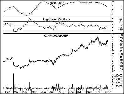
In MetaStock 6.0, it's easy to recreate the regression oscillator and the slope/close indicator from Richard Goedde's article, "Market timing with the regression oscillator," which appears in this issue. First, choose Indicator Builder from the Tools menu and enter the following formulas:
Regression Oscillator
100 * (CLOSE/ LinearReg(CLOSE,63)-1)

Slope/Close
10000* LinRegSlope(CLOSE,63)/CLOSE
Next, drag each of these formulas from the Indicator QuickList and drop them on the heading of a chart. To create horizontal lines, click the right mouse button while the mouse pointer is positioned over the regression oscillator to display the shortcut menu. Choose Regression Oscillator Properties. On the Horizontal lines page, add horizontal lines at 14, 0, and -14.

You can use The Explorer to perform the screen mentioned in the article. First, choose The Explorer from the Tools menu. Next, create a new Exploration with the following information:
Column A
Reg Osc
Fml("Regression Oscillator")

Column B
Slp/Cls
Fml("Slope/Close")

Filter
ColB > 50 and ColA >-15 and ColA < -5
Choose OK and then Explore to run the Exploration. For MetaStock for Windows 5.x users, the instructions are the same except to enter the following custom indicators in place of the ones mentioned earlier.
Regression Oscillator
100 * (CLOSE/ ((63 * Sum(Cum(1) * C,63) - Sum(Cum(1),63) * Sum(C,63))
 / (63 * Sum(Pwr(Cum(1),2),63) - Pwr(Sum(Cum(1),63),2)) * Cum(1) +
(Mov(C,63,S) - Mov(Cum(1),63,S) * (63 * Sum(Cum(1) * C,63) - Sum(Cum(1),63) * Sum(C,63)) / (63 * Sum(Pwr(Cum(1),2),63) - Pwr(Sum(Cum(1),63),2))))-1)

Slope/Close
10000* ((63 * Sum(Cum(1) * C,63) - Sum(Cum(1),63) * Sum(C,63)) / (63 * Sum(Pwr(Cum(1),2),63) - Pwr(Sum(Cum(1),63),2)))/CLOSE
-- Allan J. McNichol, EQUIS International
800 882-3040, 801 265-8886
Internet: https://www.equis.com
GO BACK
 TRADESTATION
The following functions, indicators, and system are based on the article "A new utility average stock market system" by Dennis Meyers in this issue. These analysis techniques are all written in the Power Editor in TradeStation.
We'll begin by creating the function ConsecCriteria, which is referenced by the system and the four indicators. The utility average system is based on the long/short entries specified by Meyers in his article. The four indicators graphically depict values that make up the four system entries. The names of the indicators are based on the long/short entry signal names used to identify signals within the system.
Your first step is to create the function. Please note that the Return Type for this function, which is located under the Function Properties (FILE-PROPERTIES), should be set to "TrueFalse."
Type: User Function
Name: ConsecCriteria

Inputs: Criteria(TrueFalse), Consec(Numeric);
Vars: Flag(True);

Flag = True;
For value1 = 0 To Consec - 1 Begin
  IF Criteria[value1] = False Then
     Flag = False;
End;
IF Consec = 0 Then
   Flag = False;

ConsecCriteria = Flag;
After you have created and verified the ConsecCriteria function, you can then begin work on the system and indicators. First is the code for the utility average system:
Type: System
Name: Utility Average

Inputs: Brs(3), BrsOnly(3), BCons(0), UpLag(65), Srs(-6), SrsOnly(-24), SCons(52), DnLag(100);
Vars: D1(0), D2(0), SP(0), Util(0), UtSpR(0), XCon(0), UtSpRAvg(0), UtAvg(0), UtDrB(0), UtRsB(0), UtDrS(0), UtRsS(0);

D1 = Close Data1;
D2 = Close Data2;
SP = Log(D1) * 100;
Util = Log(D2) * 100;
UtSPR = Log(D2/D1) * 100;

XCon = 2 / (1+3);
UtSpRAvg = UtSpRAvg[1] + (XCon*(UtSpR - UtSpRAvg[1]));
UtAvg = UtAvg[1] + (XCon*(Util - UtAvg[1]));
UtDrB = UtAvg - UtAvg[UpLag];
UtRsB = (UtSpRAvg - UtSpRAvg[UpLag]);
UtDrS = UtAvg - UtAvg[DnLag];
UtRsS = (UtSpRAvg - UtSpRAvg[DnLag]);

{Buy Signal}
IF (UtRsB >= Brs AND ConsecCriteria(UtDrB > 0, BCons)) Then
   Buy ("Brs&BCons") This Bar on Close;
IF UtRsB >= BrsOnly Then
   Buy ("BUtRsOnly") This Bar on Close;

{Sell Signal}
IF (UtRsS <= Srs AND ConsecCriteria(UtDrS < 0, SCons)) Then
   Sell ("Srs&SCons") This Bar on Close;
IF UtRsS <= SrsOnly Then
   Sell ("SUtRsOnly") This Bar on Close;
After creating and verifying the utility average system, you can then move on to the indicators. The first indicator is called UA - Brs&BCons, which is based on the first buy signal in the utility average system.
Type: Indicator
Name: UA - Brs&BCons

Inputs: Brs(3), BCons(0), UpLag(65);
Vars: D1(0), D2(0), SP(0), Util(0), UtSpR(0), XCon(0), UtSpRAvg(0), UtAvg(0), UtDrB(0), UtRsB(0), UtDrBSum(0);

D1 = Close Data1;
D2 = Close Data2;
SP = Log(D1) * 100;
Util = Log(D2) * 100;
UtSPR = Log(D2/D1) * 100;

XCon = 2 / (1+3);
UtSpRAvg = UtSpRAvg[1] + (XCon*(UtSpR - UtSpRAvg[1]));
UtAvg = UtAvg[1] + (XCon*(Util - UtAvg[1]));
UtDrB = UtAvg - UtAvg[UpLag];
UtRsB = (UtSpRAvg - UtSpRAvg[UpLag]);

IF UtDrB < 0 Then Begin
   IF BCons <> 0 AND ConsecCriteria(UtDrB < 0, BCons) = False Then
       UtDrBSum = UtDrBSum +1;
End Else
   UtDrBSum = 0;

Plot1(UtRsB, "UtRsB");
Plot2(UtDrBSum/10, "UtDrBSum");
Plot3(Brs, "Brs");
Plot4(0, "Zero");
Next is the UA - BUtRsOnly indicator, which is based on the second buy signal in the utility average system.
Type: Indicator
Name: UA - BUtRsOnly

Inputs: BrsOnly(3), UpLag(65);
Vars: D1(0), D2(0), SP(0), Util(0), UtSpR(0), XCon(0), UtSpRAvg(0), UtRsB(0);

D1 = Close Data1;
D2 = Close Data2;
SP = Log(D1) * 100;
Util = Log(D2) * 100;
UtSPR = Log(D2/D1) * 100;

XCon = 2 / (1+3);
UtSpRAvg = UtSpRAvg[1] + (XCon*(UtSpR - UtSpRAvg[1]));
UtRsB = (UtSpRAvg - UtSpRAvg[UpLag]);

Plot1(UtRsB, "UtRsB");
Plot2(BrsOnly, "BrsOnly");
Next is the UA - Srs&SCons indicator, which is based on the first sell signal in the utility average system.
Type: Indicator
Name: UA - SrS&Scons

Inputs: Srs(-6), SCons(52), DnLag(100);
Vars: D1(0), D2(0), SP(0), Util(0), UtSPR(0), XCon(0), UtAvg(0), UtSpRAvg(0), UtRsS(0), UtDrS(0), UtDrSSum(0);

D1 = Close Data1;
D2 = Close Data2;
SP = Log(D1) * 100;
Util = Log(D2) * 100;
UtSPR = Log(D2/D1) * 100;

XCon = 2 / (1+3);
UtSpRAvg = UtSpRAvg[1] + (XCon*(UtSpR - UtSpRAvg[1]));
UtAvg = UtAvg[1] + (XCon*(Util - UtAvg[1]));
UtDrS = UtAvg - UtAvg[DnLag];
UtRsS = (UtSpRAvg - UtSpRAvg[DnLag]);

IF UtDrS < 0 Then Begin
   IF SCons <> 0 AND ConsecCriteria(UtDrS < 0, SCons) = False Then
     UtDrSSum = UtDrSSum -1;
End Else
   UtDrSSum = 0;

Plot1(UtRsS, "UtRsS");
Plot2(UtDrSSum/10, "UtDrS");
Plot3(Srs, "Srs");
Plot4(0, "Zero");
Finally, we have the UA - SUtRsOnly indicator, which is based on the second sell signal in the utility average system.
Type: Indicator
Name: UA - SUtRsOnly

Inputs: SrsOnly(-24), DnLag(100);
Vars: D1(0), D2(0), SP(0), Util(0), UtSPR(0), XCon(0), UtSpRAvg(0), UtRsS(0), UtDrSSum(0);

D1 = Close Data1;
D2 = Close Data2;
SP = Log(D1) * 100;
Util = Log(D2) * 100;
UtSPR = Log(D2/D1) * 100;

XCon = 2 / (1+3);
UtSpRAvg = UtSpRAvg[1] + (XCon*(UtSpR - UtSpRAvg[1]));
UtRsS = (UtSpRAvg - UtSpRAvg[DnLag]);

Plot1(UtRsS, "UtRsS");
Plot2(SrsOnly, "SrsOnly");
The BUtRsOnly and SrS&SCons indicators replicate the indicators displayed in Figures 9A through 9L in Meyers's article.
This code is available at Omega's Web site. The file name is "UTIL_AVG.ELA."
-- Gaston Sanchez, Omega Research
800 422-8587, 305 270-1095
Internet: https://www/omegaresearch.com
GO BACK
 TECHNIFILTER PLUS
Here's a TechniFilter Plus trading strategy that implements Dennis Meyers's system given in "A new utility average stock market system" in this issue.
With this implementation, do not prepare the ASCII datafiles that Meyers used. This TechniFilter Plus strategy works directly with the raw data on the S&P 500 index and the Dow Jones Utility Index. The strategy uses the raw data to compute the ASCII statistics in formulas 3 and 4. Then the rules use formula 3 as the price at which to take positions. Formulas 3 through 5 are the data inputs used by Meyers. Formulas 6 through 11 compute the statistics listed in Meyers's utility model. Formula 12 is the buy condition, and formula 13 is the sell condition. The parameters listed in the formulas are the ones found by Meyers to be optimal.
Strategy Name: LOG_UTL
FORMULAS
1.  name: SPX                  format: ####.##
    formula: ~<SPX>~
2.  name: DJUA                 format: ####.##
    formula: ~<UTL>~
3.  name: SP                   format: ####.##
    formula: 100*[1]U9
4.  name: UTIL                 format: ####.##
    formula: 100*[2]U9
5.  name: UT_SP_R              format: ####.##
    formula: 100*([2]/[1])U9
6.  name: UT_SP_R_AV(3)        format: ####.##
    formula: [5]X&1
7.  name: UT_AV(3)             format: ####.##
    formula: [4]X&1
8.  name: UT_DR_B(65)          format: ####.##
    formula: [7]-TY&1
9.  name: UT_RS_B(65)          format: ####.##
    formula: [6]-TY&1
10. name: UT_DR_S(100)         format: ####.##
    formula: [7]-TY&1
11. name: UT_RS_S(100)         format: ####.##
    formula: [6]-TY&1
12. name: BUY(3,0,3)           format: ###
    formula: (([9]>=&1) & (([8]>0)F&2>=&2)) ^ ([9]>=&3)
13. name: SELL(-6,52,-24)      format: ###
    formula: (([11]<=&1) & (([10]<0)F&2>=&2)) ^ ([11]<=&3)
SIGNALS
1. BUY;F12=1
2. SELL;F13=1
RULES
1. Reverse Short to Long 1 at F3* on signal: S1
2. Reverse Long to Short 1 at F3* on signal: S2
This TechniFilter Plus strategy and those from previous issues of STOCKS & COMMODITIES can be downloaded from RTR's Web site.
-- Clay Burch, RTR Software
919 510-0608
E-mail: rtrsoft@aol.com
Internet: https://www.rtrsoftware.com
GO BACK
 SMARTRADER
In a conference held in Tokyo in spring 1990, Manning Stoller presented a technique called STARC bands. STARC bands consist of a channel surrounding a simple moving average. Like Bollinger bands, these bands will tighten in low volatility markets and widen when volatility increases. In STARC bands, average true range is used as a volatility measure.
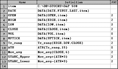
 FIGURE 1: SMARTRADER. Here's the SmarTrader code for the STARC bands.
The SmarTrader code is shown in Figure 1. Rows 9 and 10 compute the daily true range, Tr_rang and average true range (ATR). The ATR is based on 15 days but can be adjusted as desired. Row 11 is a simple moving average of the closing price. Row 12 is the STARC_Upper band and is the Mov_avg plus three times the ATR. Row 13 is the STARC_Lower band and is the Mov_avg minus three times the ATR.
The bands are plotted as lines over the bar chart.
-- Jim Ritter, Stratagem Software International
504 885-7353
E-mail: Stratagem1@aol.com
GO BACK
 WAVE WI$E MARKET SPREADSHEET
The following WAVE WI$E study implements Dennis Meyers's utility system.
A: DATE      @OMEGA(d:\omega\data\index,*DWU,Dow Utilities,D)
B: DJU
C: UTIL      @LN(DJU)*100
D: DATE      @OMEGA(d:\omega\data\index,*SPX,S&P 500 Stock Index,D)
E: sp500
F: SP        @LN(SP500)*100
G: UtSpR     @LN(DJU / SP500)*100
H: UtSpRav   @EAVG(UTSPR,3)
I: Utav      @EAVG(UTIL,3)
J: UpLag     65                       'system constant
K: DnLag     100                      'system constant
L: UtDrB     UTAV-UTAV[-UPLAG]
M: UtRsB     UtSpRav-UtSpRav[-UPLAG]
N: UtDrS     UTAV-UTAV[-DNLAG]
O: UtRsS     UTSPRAV-UTSPRAV[-DNLAG]
P: Positive  X$1=0; @IF(UTDRB>0, X$1=X$1+1 : X$1, X$1=0 : X$1)  'count up days
Q: Negative  X$1=0; @IF(UTDRS<0, X$1=X$1+1 : X$1, X$1=0 : X$1)  'count down days
R: Signal    PROCEDURE(RULES)
S:
T: colors    @IF(RULES>0, GREEN, RED)  'show the buy / sell status

'PROCEDURE RULES
#NAME BRS       3               'SYSTEM CONSTANTS
#NAME BRSONLY   3
#NAME BCONS     0
#NAME SRS       -6
#NAME SRSONLY   -24
#NAME SCONS     52
@SIGNAL(SP500,BUY,(UTRSB>=BRS & POSITIVE=BCONS) |
(UTRSB>=BRSONLY), (UTRSS<=SRS & NEGATIVE=SCONS) |
(UTRSS<=SRSONLY))
-- Peter Di Girolamo, Jerome Technology
908 369-7503
E-mail: jtiware@aol.com
Internet: https://members.aol.com/jtiware
GO BACK
Return to March Contents


![]() METASTOCK
METASTOCK ![]() TRADESTATION
TRADESTATION ![]() TECHNIFILTER PLUS
TECHNIFILTER PLUS ![]() SMARTRADER
SMARTRADER ![]() WAVE WI$E MARKET SPREADSHEET
WAVE WI$E MARKET SPREADSHEET

