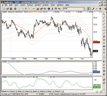
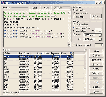
LISTING 1
// we use logarithmic returns
in =ln(Close/Ref(Close,-1));
BarsToEnd = LastValue( BarIndex() ) - BarIndex();
// calculate R/S statistics
// for last 256 bars. We divide this period into
// 1 region of 256 bars
// 2 regions of 128 bars
// 4 regions of 64 bars
// 8 regions of 32 bars
// 16 regions of 16 bars
// 32 regions of 8 bars
// (63 regions in total)
mean8 = ValueWhen( BarsToEnd % 256 == 0, MA( in, 256 ), 0 );
mean7 = ValueWhen( BarsToEnd % 128 == 0, MA( in, 128 ), 0 );
mean6 = ValueWhen( BarsToEnd % 64 == 0, MA( in, 64 ), 0 );
mean5 = ValueWhen( BarsToEnd % 32 == 0, MA( in, 32 ), 0 );
mean4 = ValueWhen( BarsToEnd % 16 == 0, MA( in, 16 ), 0 );
mean3 = ValueWhen( BarsToEnd % 8 == 0, MA( in, 8 ), 0 );
dist8 = Cum( in - mean8 ) - ValueWhen( BarsToEnd % 256 == 0, in-mean8 );
dist7 = Cum( in - mean7 ) - ValueWhen( BarsToEnd % 128 == 0, in-mean7 );
dist6 = Cum( in - mean6 ) - ValueWhen( BarsToEnd % 64 == 0, in-mean6 );
dist5 = Cum( in - mean5 ) - ValueWhen( BarsToEnd % 32 == 0, in-mean5 );
dist4 = Cum( in - mean4 ) - ValueWhen( BarsToEnd % 16 == 0, in-mean4 );
dist3 = Cum( in - mean3 ) - ValueWhen( BarsToEnd % 8 == 0, in-mean3 );
// calculate RS statistics for all regions
RS8 = ( HHV( dist8, 256 ) - LLV( dist8, 256 ) ) / StDev( in , 256 );
RS7 = ( HHV( dist7, 128 ) - LLV( dist7, 128 )) / StDev( in , 128 );
RS6 = ( HHV( dist6, 64 ) - LLV( dist6, 64 )) / StDev( in , 64 );
RS5 = ( HHV( dist5, 32 ) - LLV( dist5, 32 )) / StDev( in , 32 );
RS4 = ( HHV( dist4, 16 ) - LLV( dist4, 16 )) / StDev( in , 16 );
RS3 = ( HHV( dist3, 8 ) - LLV( dist3, 8 )) / StDev( in , 8 );
// calculate average RS is corresponding regions
ARS8 = RS8;
ARS7 = ( RS7 + Ref( RS7, -128 ) ) / 2;
ARS6 = ( RS6 +
Ref( RS6, -64 ) + Ref( RS6, -128 ) +
Ref( RS6, -192) ) / 4;
ARS5 = ( RS5 +
Ref( RS5, -32 ) + Ref( RS5, -64 ) +
Ref( RS5, -96 ) + Ref( RS5, -128 ) +
Ref( RS5, -160 ) + Ref( RS5, -192 ) +
Ref( RS5, -224 ) ) / 8;
ARS4 = ( RS4 +
Ref( RS4, -16 ) + Ref( RS4, -32 ) +
Ref( RS4, -48 ) + Ref( RS4, -64 ) +
Ref( RS4, -80 ) + Ref( RS4, -96 ) +
Ref( RS4, -112 ) + Ref( RS4, -128 ) +
Ref( RS4, -144 ) + Ref( RS4, -160 ) +
Ref( RS4, -176 ) + Ref( RS4, -192 ) +
Ref( RS4, -208 ) + Ref( RS4, -224 ) +
Ref( RS4, -240 ) ) / 16;
ARS3 = ( RS3 +
Ref( RS3, -8 ) + Ref( RS3, -16 ) +
Ref( RS3, -24 ) + Ref( RS3, -32 ) +
Ref( RS3, -40 ) + Ref( RS3, -48 ) +
Ref( RS3, -56 ) + Ref( RS3, -64 ) +
Ref( RS3, -72 ) + Ref( RS3, -80 ) +
Ref( RS3, -88 ) + Ref( RS3, -96 ) +
Ref( RS3, -104 ) + Ref( RS3, -112 ) +
Ref( RS3, -120 ) + Ref( RS3, -128 ) +
Ref( RS3, -136 ) + Ref( RS3, -144 ) +
Ref( RS3, -152 ) + Ref( RS3, -160 ) +
Ref( RS3, -168 ) + Ref( RS3, -176 ) +
Ref( RS3, -184 ) + Ref( RS3, -192 ) +
Ref( RS3, -200 ) + Ref( RS3, -208 ) +
Ref( RS3, -216 ) + Ref( RS3, -224 ) +
Ref( RS3, -232 ) + Ref( RS3, -240 ) +
Ref( RS3, -248 ) ) / 32;
// calculate Hurst exponent as a linear regression slope
// of Log2( AvgRS )/ Log2( region size )
Y8 = log( ARS8 )/log( 2 );
Y7 = log( ARS7 )/log( 2 );
Y6 = log( ARS6 )/log( 2 );
Y5 = log( ARS5 )/log( 2 );
Y4 = log( ARS4 )/log( 2 );
Y3 = log( ARS3 )/log( 2 );
Sumx = 3+4+5+6+7+8; // sum of log2( region size )
Sumy = Y8 + Y7 + Y6 + Y5 + Y4 + Y3; // sum of log2( AvgRS )
sumxy = 8*Y8 + 7*Y7 + 6*Y6 + 5*Y5 + 4*Y4 + 3*Y3;
Sumx2 = 3*3 + 4*4 + 5*5 + 6*6 + 7*7 + 8*8;
// the slope of linear regression from R/S
// is the estimate of Hurst exponent
b=( 6 * sumxy - sumx*sumy )/( 6 * sumx2 - sumx*sumx);
Hurst = b;
Filter = BarsToEnd == 0;
AddColumn( Close, "Close", 1.5 );
AddColumn( Hurst, "Hurst Exponent", 1.5);
AddColumn( 2-Hurst, "Fractal Dim", 1.5 );
A downloadable version of this formula is available from the
AmiBroker website.
--Tomasz Janeczko, AmiBroker.com
www.amibroker.com
GO BACK
 WEALTH-LAB: TIME AND MONEY CHARTS
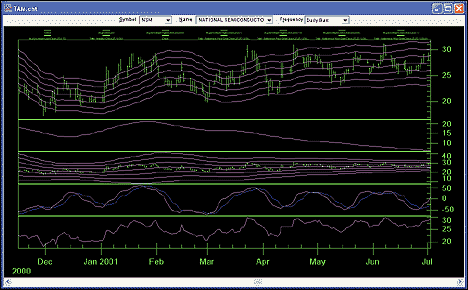
The Wealth-Lab script given here reproduces the time and money (TAM)
charts described in Stuart Belknap's article in this issue. The
reference price grid (signal) displays volatility bands at various levels
around price. When prices hit the outer band, this represents instances
where prices are reaching statistically extreme levels.
We coded a simple trading system that goes long when prices touch the
lower band and exits the position when prices reach the "norm"
(moving average).
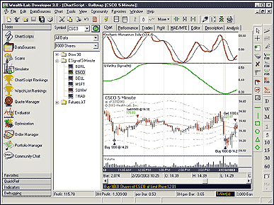
Figure 3 displays a TAM chart of Cisco five-minute bars with
this simple trading system applied.

FIGURE 3: WEALTH-LAB, TIME AND MONEY CHARTS. This sample
Wealth-Lab chart displays a TAM chart of Cisco five-minute bars with a
simple trading system applied. The system goes long when prices touch the
lower band and exits the position when prices reach the "norm"
(moving average). The chart also displays the volatility sigma (%) and
the stochastic momentum index indicator as described in Belknap's
article.
Our chart also displays the volatility sigma (%) and the stochastic momentum
index indicator as described in the article.
{$I 'SMI'}
{ Delare Variables }
var i, arm, Bar, som, yom, varyom, volPane, yomsqr, SPane: integer;
var channels: array[1..6] of integer;
var sigom, limit: float;
{ Create Custom Price Series }
arm := SMASeries( #Close, 25 );
som := CreateSeries;
yom := CreateSeries;
varyom := CreateSeries;
for i := 1 to 6 do
  channels[i] := CreateSeries;
{ Populate YOM Series }
for Bar := 60 to BarCount - 1 do
  @yom[Bar] := 100 * ( PriceClose( Bar ) - @arm[Bar - 12] ) / @arm[Bar - 12];
yomsqr := MultiplySeries( yom, yom );
{ Populate SOM Series }
for Bar := 60 to BarCount - 1 do
begin
  @varyom[Bar] := Sum( Bar, yomsqr, 50 ) / 50;
  @som[Bar] := Sqrt( @varyom[Bar] );
end;
{ Populate Reference Price Grids }
for Bar := 60 to BarCount - 1 do
begin
  sigom := SMA( Bar, som, 25 );
  for i := 1 to 3 do
  begin
    SetSeriesValue( Bar, channels[i], ( 1 + i * sigom / 100 ) * @arm[Bar] );
    SetSeriesValue( Bar, channels[i + 3], ( 1 - i * sigom / 100 ) *
@arm[Bar] );
  end;
end;
{ Plot Reference Price Grids }
PlotSeries( arm, 0, #Gray, #Thin );
for i := 1 to 6 do
  PlotSeries( channels[i], 0, #Gray, #Dotted );
{ Populate Volatility Sigma }
VolPane := CreatePane( 100, true, true );
PlotSeries( SMASeries( som, 25 ), VolPane, 060, #Thick );
DrawLabel( 'Volatility Sigma(%)', VolPane );
{ Plot Stochastic Momentum Index }
SPane := CreatePane( 100, true, true );
PlotSeries( SMISeries( 12, 6, 6 ), SPane, #Maroon, #Thick );
PlotSeries( SMASeries( SMISeries( 12, 6, 6 ), 6 ), SPane, #Black, #Thin );
DrawLabel( 'Stochastic Momentum Index(12,6,6)', SPane );
{ Simple Trading Rules }
for Bar := 100 to BarCount - 1 do
begin
  if MarketPosition = 0 then
  begin
    limit := GetSeriesValue( Bar, channels[6] );
    BuyAtLimit( Bar + 1, limit, '' );
  end
  else
    SellAtLimit( Bar + 1, @arm[Bar], LastPosition, '' );
end;
--Dion Kurczek, Wealth-Lab, Inc.
www.wealth-lab.com
GO BACK
 WEALTH-LAB: FRACTAL DIMENSION INDEX
In his article "Making Sense Of Fractals," Erik Long uses
the Hurst exponent as a basis for his fractal dimension index (FDI) indicator.
The Hurst exponent measures the smoothness of a fractal time series based
on the asymptotic behavior of its rescaled range. A value of 0.50 indicates
that the time series behaves very closely to a random walk. Values higher
than 0.50 indicate that the price series covers more distance than a random
walk, and values less than 0.50 indicate less distance.
The Wealth-Lab script here calculates the Hurst exponent based on a
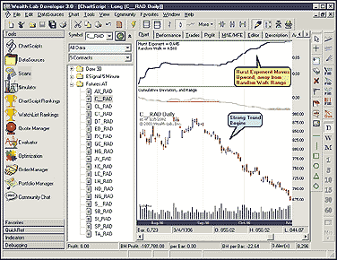
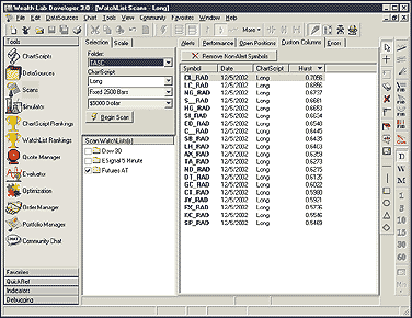
sliding 200-bar sample window. Figure 4 displays the Hurst
exponent for daily corn futures. Figure 5 shows the tabular results.
Note how the Hurst exponent moves away from 0.50 as prices start forming
a strong trend.

FIGURE 4: WEALTH-LAB, HURST EXPONENT. This sample Wealth-Lab
chart displays the Hurst exponent for daily corn futures. Note how the
Hurst exponent moves away from 0.50 as prices start forming a strong trend.

FIGURE 5: WEALTH-LAB, HURST EXPONENT. Here are the tabular results
for the chart displayed in Figure 4.
{ Declare Variables }
var E, Hurst, Bar, Period, SumDiff, FDIPane, EPane: integer;
var R, S, H: float;
Period := 200;
{ Create Custom Indicator Series }
Hurst := CreateSeries;
E := CreateSeries;
{ Our "E" Series is P/P[-1] }
for Bar := 1 to BarCount - 1 do
  @E[Bar] := PriceClose( Bar ) / PriceClose( Bar - 1 );
{ Calculate the sum of deviations over the period }
SumDiff := SumSeries( SubtractSeries( E, SMASeries( E, Period ) ), Period );
{ Plot deviation range }
EPane := CreatePane( 50, true, true );
HidePaneLines;
PlotSeries( HighestSeries( SumDiff, Period ), EPane, 474, #Thick );
PlotSeries( LowestSeries( SumDiff, Period ), EPane, 744, #Thick );
PlotSeries( SumDiff, EPane, #Silver, #Thick );
DrawLabel( 'Cumulative Deviation, and Range', EPane );
{ Calculate R/S and the Hurst Exponent }
for Bar := Period * 2 to BarCount - 1 do
begin
  R := Highest( Bar, SumDiff, Period ) - Lowest( Bar, SumDiff, Period );
  S := StdDev( Bar, E, Period );
  @Hurst[Bar] := LN( R / S ) / LN( Period );
end;
{ Plot Hurst Exponent }
FDIPane := CreatePane( 100, true, true );
PlotSeries( Hurst, FDIPane, #Navy, #Thick );
H := @Hurst[BarCount - 1];
DrawLabel( 'Hurst Exponent = ' + FormatFloat( '#0.000', H ), FDIPane );
DrawLabel( 'Random Walk = 0.500', FDIPane );
AddScanColumnStr( 'Hurst', FormatFloat( '#0.0000', @Hurst[BarCount - 1] ) );
--Dion Kurczek, Wealth-Lab, Inc.
www.wealth-lab.com
GO BACK
 NEUROSHELL TRADER: TIME AND MONEY CHARTS
In this issue, Stuart Belknap describes several indicators that are
either already built into NeuroShell Trader Professional or can be recreated
by combining a few of the 800-plus technical indicators already in NeuroShell.
We've combined all the relevant indicators to recreate Belknap's
indicators. These indicators are in a chart that can be downloaded from
the NeuroShell Trader free technical support website.
To insert Belknap's channel lines:
1. Select "New Indicator ..." from
the Insert menu
2. Select the Simple Moving Average category
3. Select the simple moving average, simple moving average envelope
high, and simple moving average envelope low
4. Select the simple moving average envelope high parameter "envelope
fraction"
5. Press the Set Parameter button and set the parameter to 0.03,0.02,0.01
6. Select the simple moving average envelope low parameter "envelope
fraction"
7. Press the Set Parameter button and set the parameter to 0.03,0.02,0.01
8. Select the Finished button
To add the other custom indicators to your chart:
1. Select "New Indicator ..." from the Insert
menu
2. Select the Custom Indicator category
3. Select the TAM--volatility, TAM--reference price grid,
and TAM--stochastic momentum indicators
4. Select the TAM ? reference price grid parameter "envelope
fraction"
5. Press the Set Parameter button and set the parameter to -0.03,-0.02,-0.01,0.0.01,0.02,0.03
(this will provide you with the entire grid as Belknap suggests)
6. Select the Finished button.
To insert Belknap's average bar price:
1. Select "New Indicator ..." from the Insert
menu.
2. Select the Arithmetic category.
3. Select the Average2.
4. Set the Operand #1 and Operand #2 parameters to High and Low, respectively.
5. Select the Finished button.
You can easily insert any of these indicators into a prediction or trading
strategy (however, do not trade with Belknap's TAM volatility or
Tam reference grid indicators, since they look ahead in time). The coefficients
can be optimized by the genetic algorithm built into NeuroShell Trader
Professional or DayTrader Professional. This can provide you with custom
versions of Belknap's indicators that perform best with your favorite
issues.
Users of NeuroShell Trader can go to the STOCKS & COMMODITIES section
of the NeuroShell Trader free technical support website to download a sample
chart (Figure 6) implementing this tip.

FIGURE 6: NEUROSHELL TRADER,TIME AND MONEY CHART. Here's
a sample NeuroShell Trader chart demonstrating Belknap's indicators.
For more information on NeuroShell Trader, visit www.NeuroShell.com.
--Marge Sherald, Ward Systems Group, Inc.
301 662-7950, sales@wardsystems.com
www.neuroshell.com
GO BACK
 NEUROSHELL TRADER: FRACTAL DIMENSION INDEX
Erik Long's fractal dimension index (FDI) can be easily implemented
in NeuroShell Trader Professional by using the Hurst exponent indicator.
This indicator is available from the NeuroShell Advanced Indicator Set
1 extra-cost add-on, in addition to using standard indicators included
with NeuroShell Trader software.
First, insert the standard subtract indicator by doing the following:
1. Select "New Indicator ..." from the Insert
menu.
2. Select the Arithmetic category.
3. Select the Subtract indicator.
4. Set Operand #1 equal to 2.
5. Set Operand #2 to the Hurst exponent indicator in the Advanced Indicator
Set 1 category.
6. Select the Finished button.
7. Right-click on the completed indicator and rename it to FDI (fractal
dimension index).
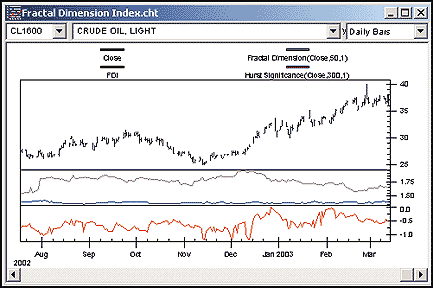
Note that for additional study, we also added to our chart the Hurst significance
and fractal dimension indicators from the Advanced Indicator Set 1 add-on
(Figure 7).

FIGURE 7: NEUROSHELL TRADER, FRACTAL DIMENSION INDEX.
Here's a sample NeuroShell Trader chart demonstrating the fractal
dimension index with related indicators.
If you decide to use your indicator in a trading strategy, the coefficients
may be optimized by the Genetic Algorithm built into the NeuroShell Trader
Professional. This can provide you with the parameters that maximize profitability.
Users of NeuroShell Trader can go to the STOCKS & COMMODITIES section
of the NeuroShell Trader free technical support website to download a sample
NeuroShell chart implementing this tip.
For more information on NeuroShell Trader, visit www.NeuroShell.com.
--Marge Sherald, Ward Systems Group, Inc.
301 662-7950, sales@wardsystems.com
www.neuroshell.com
GO BACK
 NEOTICKER: TIME AND MONEY CHARTS
To construct the TAM charts presented in "Time And Money Charts"
by Stuart Belknap in NeoTicker, first construct four indicators: Channel
Lines (Listing 1), Volatility (Listing 2), Reference Price Grid (Listing
3) and Stochastic Momentum Index (Listing 4). Then apply those indicators
to the different time frame charts.
LISTING 1
Channel Lines
mycount := mycount +1;
xarm := average(data1, 25);
xdel := 5;
plot1 := (1+1*xdel/100)*xarm;
plot2 := (1+2*xdel/100)*xarm;
plot3 := (1+3*xdel/100)*xarm;
plot4 := (1-1*xdel/100)*xarm;
plot5 := (1-2*xdel/100)*xarm;
plot6 := (1-3*xdel/100)*xarm;
plot7 := xarm;
cond :=  if (mycount > 25, 1, 0);
success1 := cond;
success2 := cond;
success3 := cond;
success4 := cond;
success5 := cond;
success6 := cond;
success7 := cond;
LISTING 2
Volatility
mycount := mycount+1;
yom := 100*(close(12)-average(data1,25))/average(data1,25);
avyom := summation(yom,50)/50;
varyom := (summation(yom*yom,50)/50)-(avyom*avyom);
som := sqrt(varyom);
plot1 := average(som,25);
success1 := if (mycount > 25, 1, 0);
LISTING 3
Reference Price Grid
myarm := average(data1,25);
mycount := mycount+1;
plot1 := (1+1*sigom(data1)/100)*myarm;
plot2 := (1+2*sigom(data1)/100)*myarm;
plot3 := (1+3*sigom(data1)/100)*myarm;
plot4 := (1-1*sigom(data1)/100)*myarm;
plot5 := (1-2*sigom(data1)/100)*myarm;
plot6 := (1-3*sigom(data1)/100)*myarm;
plot7 := myarm;
cond :=  if (mycount > 25, 1, 0);
success1 := cond;
success2 := cond;
success3 := cond;
success4 := cond;
success5 := cond;
success6 := cond;
success7 := cond;
LISTING 4
Stochastic Momentum Index
q := param1;
r := param2;
s := param3;
i := param4;
myms := close - 0.5*(hhv(data1.h, q)+llv(data1.l, q));
mydiff := (hhv(data1.h, q)-llv(data1.l, q));
StochMoIdx := 100*qc_xaverage(qc_xaverage(myms,r),s)/
              (0.5*qc_xaverage(qc_xaverage(mydiff,r),s));
plot1 := StochMoIdx;
plot2 := average(StochMoIdx, i);
plot3 := 50;
plot4 := -50;
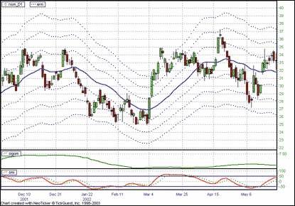
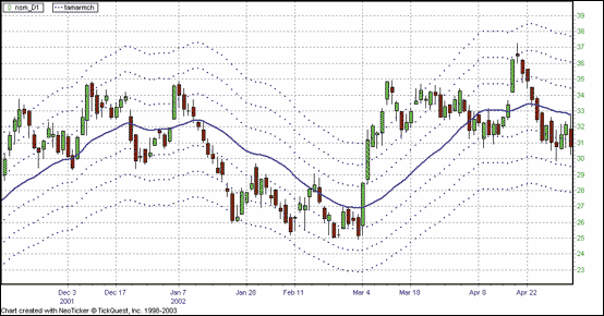
To create the daily TAM charts, open a daily chart, expand the numbers
of days to load to 100, then add the volatility sigma, stochastic momentum,
and price reference on the chart to get the daily TAM chart (Figure
8).

FIGURE 8: NEOTICKER, DAILY TIME AND MONEY CHART. Add
the volatility sigma, stochastic momentum, and price reference on the NeoTicker
chart to get the daily TAM chart.
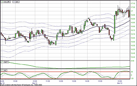
For intraday TAM charts, change the days to load to "5"
and change the bar type to "minute" and size to "5,"
to make the chart into a five-minute chart (Figure 9).

FIGURE 9: NEOTICKER,FIVE-MINUTE TIME AND MONEY CHART.
For intraday TAM charts, change the days to load to "5" and
change the bar type to "minute" and size to "5"
to make the chart into a five-minute chart.
Use the price channels lines indicator to create the candlestick chart
that demonstrates price action using the moving average and its offset
channels (Figure 10), as described in Long's article.

FIGURE 10: NEOTICKER,CANDLESTICK TIME AND MONEY CHART.
Use the price channels lines indicator to create the candlestick chart
that demonstrates price action using the moving average and its offset
channels, as described in Long's article.
A downloadable version of the indicators is available from the Yahoo!
NeoTicker user group file area at https://groups.yahoo.com/group/neoticker/.
--Kenneth Yuen, TickQuest Inc.
www.tickquest.com
GO BACK
 NEOTICKER: FRACTAL DIMENSION INDEX
The fractal dimension index (FDI) presented in "Making Sense
Of Fractals" by Erik Long in this issue can be implemented in NeoTicker
using VBScript.
Start by creating a new indicator and name it "FDI" (Listing
1) with one integer parameter Period. Input the following code:
LISTING 1
function fdi()
dim n, i, j, k, l, ydiff, dy, dx2, lgth
dim ymin, ymax
   n = param1.int
   if heap.size = 0 then
      heap.allocate (n+1)
      heap.fill 0, n, 0
   end if
   if not data1.valid (0) then
      itself.success = false
      exit function
   end if
   i = heap.value(n) mod n
   heap.value (i) = data1.value (0)
   heap.inc (n)
   if heap.value (n) < n then
      itself.success = false
      exit function
   end if
   ymin = heap.min (0, n-1)
   ymax = heap.max (0, n-1)
   ydiff = ymax-ymin
   dx2 = tq_power ((1/(n-1)), 2)
   for j = 1 to n-1
      k = (i+j) mod n
      l = (i+j+1) mod n
      dy = (heap.value (k)-heap.value (l))/ydiff
      lgth = lgth + tq_sqrt(dx2 + dy*dy)
   next
   fdi = 1 + (tq_log10(lgth) + tq_log10(2))/tq_log10(2*(n-1))
end function
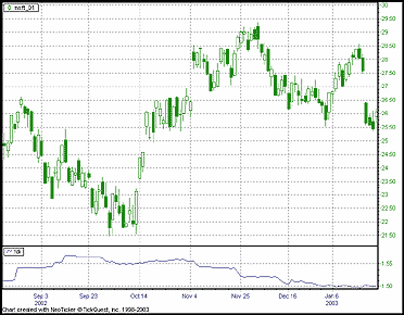
The FDI indicator, when added to a chart, will return the
fractal dimension index of the underlying instruments (Figure 11).
A downloadable version of this indicator is available from the
Yahoo! NeoTicker user group file area at https://groups.yahoo.com/group/neoticker/.

FIGURE 11: NEOTICKER, FRACTAL DIMENSION INDEX. Here's
a sample NeoTicker chart of the FDI (bottom pane) with the underlying instrument
(top pane).
AMIBROKER: TIME AND MONEY CHARTS
AMIBROKER: FRACTAL DIMENSION INDEX
WEALTH-LAB: TIME AND MONEY CHARTS
WEALTH-LAB: FRACTAL DIMENSION INDEX
NEUROSHELL TRADER: TIME AND MONEY CHARTS
NEUROSHELL TRADER: FRACTAL DIMENSION INDEX
NEOTICKER: TIME AND MONEY CHARTS
NEOTICKER: FRACTAL DIMENSION INDEX
ASPEN GRAPHICS: TIME AND MONEY CHARTS
STOCKWIZ: FRACTAL DIMENSION INDEX
METASTOCK
![]() AMIBROKER: TIME AND MONEY CHARTS
AMIBROKER: TIME AND MONEY CHARTS
