TRADERS’ TIPS
November 2009
Here is this month’s selection of Traders’ Tips, contributed by various developers of technical analysis software to help readers more easily implement some of the strategies presented in this and other issues.
Other code appearing in articles in this issue is posted in the Subscriber Area of our website at https://technical.traders.com/sub/sublogin.asp. Login requires your last name and subscription number (from mailing label). Once logged in, scroll down to beneath the “Optimized trading systems” area until you see “Code from articles.” From there, code can be copied and pasted into the appropriate technical analysis program so that no retyping of code is required for subscribers.
You can copy these formulas and programs for easy use in your spreadsheet or analysis software. Simply “select” the desired text by highlighting as you would in any word processing program, then use your standard key command for copy or choose “copy” from the browser menu. The copied text can then be “pasted” into any open spreadsheet or other software by selecting an insertion point and executing a paste command. By toggling back and forth between an application window and the open web page, data can be transferred with ease.
This month’s tips include formulas and programs for:
- TRADESTATION: SEASONAL CHANNEL BREAKOUT SYSTEM
- eSIGNAL: SEASONAL CHANNEL BREAKOUT SYSTEM
- WEALTH-LAB: SEASONAL CHANNEL BREAKOUT SYSTEM
- AMIBROKER: SEASONAL CHANNEL BREAKOUT SYSTEM
- NEUROSHELL TRADER: SEASONAL CHANNEL BREAKOUT SYSTEM
- AIQ: SEASONAL CHANNEL BREAKOUT SYSTEM
- TRADERSSTUDIO: SEASONAL CHANNEL BREAKOUT SYSTEM
- TRADECISION: SEASONAL CHANNEL BREAKOUT SYSTEM
- TRADE NAVIGATOR: SEASONAL CHANNEL BREAKOUT SYSTEM
- NINJATRADER: SEASONAL CHANNEL BREAKOUT SYSTEM
- UPDATA: SEASONAL CHANNEL BREAKOUT SYSTEM
- UPDATA: THE PIVOT DETECTOR OSCILLATOR, SIMPLIFIED
- VT TRADER: FOUR-PERIOD LOOKBACK %R PAINTBAR SYSTEM
- TRADE IDEAS: SEASONAL CHANNEL BREAKOUT SYSTEM
- MULTICHARTS: SOYBEAN SEASONAL CHANNEL BREAKOUT SYSTEM (KATSANOS ARTICLE CODE)
![]() TRADESTATION: SEASONAL CHANNEL BREAKOUT SYSTEM
TRADESTATION: SEASONAL CHANNEL BREAKOUT SYSTEM
Markos Katsanos’ article in this issue, “A Seasonal System For Trading Soybean Futures,” starts with an inflation-adjusted seasonal analysis of daily soybean-future price activity since 1995. From this, Katsanos extracts the basic trading rule: short in June or July, buy any other month except August. This insight is then combined with two different trading strategies: a simple seasonal breakout that buys in September and shorts in June, and one that combines seasonal bias with moving average crossover signals coming from daily dollar index and soybean price activity. Finally, a simple moving average crossover system based entirely on daily soy price action is provided for comparison purposes.
For this second system, Katsanos provides his daily, inflation-adjusted cycle data in the form of a text file. This can be imported directly (with provided soy and dollar data) to reproduce the published results. To provide for real-time testing of the system, the seasonal cycle information was placed in a function. Code for this function and an adapted strategy using it are provided here.
A sample chart implementing the systems in TradeStation is shown in Figure 1.
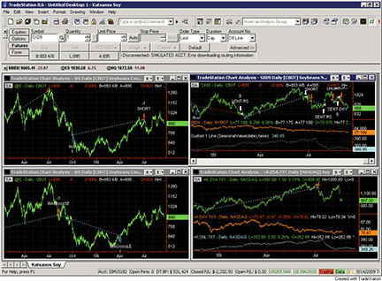
Figure 1: TRADESTATION, Katsanos’ Seasonal Soybean systems. Shown in the lower-left subgraph is Markos Katsanos’ simple crossover system trading the continuous soybean futures contract. In the upper-left subgraph is Markos Katsanos’ simple seasonal signal. The upper-right subgraph shows the seasonal breakout with dollar and soy crossover signals modified to use real-time data. The lower-right subgraph shows the seasonal soybean signal with crossover, using imported ASCII data from Katsanos.
To download the adapted EasyLanguage code, Katsanos’ code, and Katsanos’ data files, go to the TradeStation and EasyLanguage Support Forum (https://www.tradestation.com/Discussions/forum.aspx?Forum_ID=213). Search for the file “SeasonalSoy.eld.”
This article is for informational purposes. No type of trading or investment recommendation, advice, or strategy is being made, given or in any manner provided by TradeStation Securities or its affiliates.
Strategy: SeasonalSoyCrossMod
  {*************************************
  Modified Soybean Seasonal-Channel Breakout Strategy
  Based on work by MARKOS KATSANOS
  Data3 references replaced by the function SeasonalValues
  **************************************}
{Length=Channel Length in days,
  D1DXY=Days for the Dollar Index linear regression slope calculation
  D2SNL=Days for the Seasonal data linear regression slope calculation
  LRSNLSELL= Seasonal data linear regression slope per day
  LRSDXYSELL=Dollar index linear regression slope per day
  MASNL=Days for the seasonal exponential moving average sell/
  buytocover conditions
  MASELL=Days for the Soybean exponential moving average sell/
  buytocover conditions
  MADXY=Days for the Dollar Index moving average sell/buytocover
  conditions}
inputs:
  Length(4),
  D1DXY(25),
  D2SNL(12),
  SellMonth(6),
  BuyMonth(9),
  LRSNLSELL(-.8),
  LRSDXYSELL(.3),
  MASNL(15),
  MASELL(15),
  MADXY(50) ;
  variables:
  RS(0),
  LRSNL(0),
  S2(0),
  STOPL(0),
  SeasonalBuy(FALSE),
  SEASONALSHORT(FALSE),
  LRSDXY(0) ;
  IF BarNumber>3 then
  BEGIN
  RS=XAverage((Close / SeasonalValue( Date )),3) ;
  END;
  IF BarNumber>D2SNL+3 then
  BEGIN
  LRSNL=(LinearRegValue(RS,D2SNL,0)
  - LinearRegValue(RS,D2SNL,D2SNL))
  / LinearRegValue(RS,D2SNL,D2SNL)
  / D2SNL*100;
  END;
  IF BarNumber>D1DXY then
  BEGIN
  LRSDXY=(LinearRegValue(Close Data2,D1DXY,0)
  - LinearRegValue(Close Data2,D1DXY,D1DXY))
  / LinearRegValue(Close Data2,D1DXY,D1DXY)
  / D1DXY*100;
  END;
  SeasonalBuy=Month( Date )<SellMonth
  OR Month( Date )>BuyMonth;
  SEASONALSHORT=MONTH( Date )>SellMonth and
  MONTH( Date )< BuyMonth + 1;
  {Buy&Short conditions}
  IF SeasonalBuy and LRSDXY<LRSDXYSELL
  and Close >( Highest(Close[1],Length)+2)
  and LRSNL>LRSNLSELL
  then
  Buy ( “Buy” ) next bar market;
  IF SEASONALSHORT
  and C<LOWEST(C,Length)[1]-2
  and LRSDXY>-LRSDXYSELL
  and LRSNL<-LRSNLSELL
  then
  sellshort (“SHORT”) next bar at market;
  {Exit conditions}
  IF marketposition=1
  and barssinceentry>1
  then
  begin
  IF C<XAverage(C,MASELL)
  and LRSNL<LRSNLSELL
  then
  SELL(“LEXIT RS”) NEXT BAR AT OPEN; {RS with SNL Exit}
  IF C<XAverage(C,MASELL)
  and XAverage(Close Data2,MADXY)
  > XAverage(Close Data2,MADXY)[1]
  and LRSDXY>LRSDXYSELL then
  Sell (“LEXIT DXY”) next bar at market;
  {DXY Exit}
  END;
  IF marketposition=-1 and barssinceentry>1 then
  begin
  IF C>XAverage(C,MASELL)
  and LRSNL>-LRSNLSELL
  then
  buytocover (“SEXIT RS”) next bar at market;
  IF C>XAverage(C,MASELL)
  and XAverage(Close Data2,MADXY)
  < XAverage(Close Data2,MADXY)[1]
  and SeasonalValue( Date )
  > XAverage(SeasonalValue( Date ),MASNL)
  then
  buytocover (“SEXIT DXY”)next bar at market;
  END;
Function: SeasonalValue
  Inputs:
  SpecificDate( numeric ) ;
  variables:
  Int MonthDay(0) ;
  MonthDay = Date - IntPortion(Date/10000)*10000 ;
  switch( MonthDay )
  Begin
  Case 101: SeasonalValue = 355.060 ; // Jan-01
  Case 102: SeasonalValue = 357.130 ; // Jan-02
  Case 103: SeasonalValue = 357.095 ; // Jan-03
  Case 104: SeasonalValue = 357.060 ; // Jan-04
  Case 105: SeasonalValue = 357.610 ; // Jan-05
  Case 106: SeasonalValue = 357.160 ; // Jan-06
  Case 107: SeasonalValue = 357.780 ; // Jan-07
  Case 108: SeasonalValue = 357.600 ; // Jan-08
  Case 109: SeasonalValue = 357.130 ; // Jan-09
  Case 110: SeasonalValue = 356.430 ; // Jan-10
  Case 111: SeasonalValue = 356.790 ; // Jan-11
  Case 112: SeasonalValue = 358.670 ; // Jan-12
  Case 113: SeasonalValue = 360.090 ; // Jan-13
  Case 114: SeasonalValue = 359.510 ; // Jan-14
  Case 115: SeasonalValue = 359.730 ; // Jan-15
  Case 116: SeasonalValue = 358.350 ; // Jan-16
  Case 117: SeasonalValue = 358.450 ; // Jan-17
  Case 118: SeasonalValue = 357.630 ; // Jan-18
  Case 119: SeasonalValue = 357.950 ; // Jan-19
  Case 120: SeasonalValue = 358.480 ; // Jan-20
  Case 121: SeasonalValue = 359.020 ; // Jan-21
  Case 122: SeasonalValue = 357.700 ; // Jan-22
  Case 123: SeasonalValue = 355.980 ; // Jan-23
  Case 124: SeasonalValue = 358.220 ; // Jan-24
  Case 125: SeasonalValue = 357.910 ; // Jan-25
  Case 126: SeasonalValue = 358.110 ; // Jan-26
  Case 127: SeasonalValue = 358.710 ; // Jan-27
  Case 128: SeasonalValue = 357.540 ; // Jan-28
  Case 129: SeasonalValue = 358.130 ; // Jan-29
  Case 130: SeasonalValue = 359.440 ; // Jan-30
  Case 131: SeasonalValue = 358.440 ; // Jan-31
  Case 201: SeasonalValue = 356.520 ; // Feb-01
  Case 202: SeasonalValue = 356.610 ; // Feb-02
  Case 203: SeasonalValue = 357.070 ; // Feb-03
  Case 204: SeasonalValue = 359.520 ; // Feb-04
  Case 205: SeasonalValue = 359.860 ; // Feb-05
  Case 206: SeasonalValue = 359.310 ; // Feb-06
  Case 207: SeasonalValue = 359.570 ; // Feb-07
  Case 208: SeasonalValue = 359.020 ; // Feb-08
  Case 209: SeasonalValue = 360.230 ; // Feb-09
  Case 210: SeasonalValue = 360.270 ; // Feb-10
  Case 211: SeasonalValue = 360.350 ; // Feb-11
  Case 212: SeasonalValue = 359.720 ; // Feb-12
  Case 213: SeasonalValue = 360.910 ; // Feb-13
  Case 214: SeasonalValue = 363.310 ; // Feb-14
  Case 215: SeasonalValue = 364.070 ; // Feb-15
  Case 216: SeasonalValue = 364.250 ; // Feb-16
  Case 217: SeasonalValue = 365.700 ; // Feb-17
  Case 218: SeasonalValue = 367.100 ; // Feb-18
  Case 219: SeasonalValue = 368.290 ; // Feb-19
  Case 220: SeasonalValue = 369.410 ; // Feb-20
  Case 221: SeasonalValue = 369.780 ; // Feb-21
  Case 222: SeasonalValue = 370.120 ; // Feb-22
  Case 223: SeasonalValue = 369.920 ; // Feb-23
  Case 224: SeasonalValue = 369.220 ; // Feb-24
  Case 225: SeasonalValue = 371.880 ; // Feb-25
  Case 226: SeasonalValue = 371.860 ; // Feb-26
  Case 227: SeasonalValue = 372.050 ; // Feb-27
  Case 228: SeasonalValue = 374.480 ; // Feb-28
  Case 229: SeasonalValue = 373.895 ; // Feb-29
  Case 301: SeasonalValue = 373.310 ; // Mar-01
  Case 302: SeasonalValue = 373.370 ; // Mar-02
  Case 303: SeasonalValue = 375.820 ; // Mar-03
  Case 304: SeasonalValue = 373.110 ; // Mar-04
  Case 305: SeasonalValue = 372.540 ; // Mar-05
  Case 306: SeasonalValue = 372.070 ; // Mar-06
  Case 307: SeasonalValue = 369.820 ; // Mar-07
  Case 308: SeasonalValue = 369.610 ; // Mar-08
  Case 309: SeasonalValue = 371.510 ; // Mar-09
  Case 310: SeasonalValue = 372.340 ; // Mar-10
  Case 311: SeasonalValue = 374.770 ; // Mar-11
  Case 312: SeasonalValue = 372.840 ; // Mar-12
  Case 313: SeasonalValue = 373.350 ; // Mar-13
  Case 314: SeasonalValue = 371.900 ; // Mar-14
  Case 315: SeasonalValue = 372.980 ; // Mar-15
  Case 316: SeasonalValue = 373.300 ; // Mar-16
  Case 317: SeasonalValue = 370.920 ; // Mar-17
  Case 318: SeasonalValue = 371.110 ; // Mar-18
  Case 319: SeasonalValue = 369.730 ; // Mar-19
  Case 320: SeasonalValue = 368.040 ; // Mar-20
  Case 321: SeasonalValue = 367.250 ; // Mar-21
  Case 322: SeasonalValue = 369.450 ; // Mar-22
  Case 323: SeasonalValue = 368.770 ; // Mar-23
  Case 324: SeasonalValue = 369.130 ; // Mar-24
  Case 325: SeasonalValue = 372.190 ; // Mar-25
  Case 326: SeasonalValue = 373.320 ; // Mar-26
  Case 327: SeasonalValue = 373.760 ; // Mar-27
  Case 328: SeasonalValue = 372.200 ; // Mar-28
  Case 329: SeasonalValue = 372.860 ; // Mar-29
  Case 330: SeasonalValue = 373.810 ; // Mar-30
  Case 331: SeasonalValue = 368.540 ; // Mar-31
  Case 401: SeasonalValue = 369.900 ; // Apr-01
  Case 402: SeasonalValue = 373.070 ; // Apr-02
  Case 403: SeasonalValue = 371.250 ; // Apr-03
  Case 404: SeasonalValue = 369.980 ; // Apr-04
  Case 405: SeasonalValue = 369.870 ; // Apr-05
  Case 406: SeasonalValue = 368.580 ; // Apr-06
  Case 407: SeasonalValue = 370.410 ; // Apr-07
  Case 408: SeasonalValue = 368.710 ; // Apr-08
  Case 409: SeasonalValue = 370.980 ; // Apr-09
  Case 410: SeasonalValue = 372.630 ; // Apr-10
  Case 411: SeasonalValue = 370.980 ; // Apr-11
  Case 412: SeasonalValue = 370.550 ; // Apr-12
  Case 413: SeasonalValue = 371.480 ; // Apr-13
  Case 414: SeasonalValue = 374.860 ; // Apr-14
  Case 415: SeasonalValue = 373.300 ; // Apr-15
  Case 416: SeasonalValue = 371.230 ; // Apr-16
  Case 417: SeasonalValue = 373.120 ; // Apr-17
  Case 418: SeasonalValue = 375.130 ; // Apr-18
  Case 419: SeasonalValue = 375.820 ; // Apr-19
  Case 420: SeasonalValue = 375.740 ; // Apr-20
  Case 421: SeasonalValue = 373.630 ; // Apr-21
  Case 422: SeasonalValue = 375.480 ; // Apr-22
  Case 423: SeasonalValue = 376.060 ; // Apr-23
  Case 424: SeasonalValue = 376.210 ; // Apr-24
  Case 425: SeasonalValue = 377.380 ; // Apr-25
  Case 426: SeasonalValue = 376.690 ; // Apr-26
  Case 427: SeasonalValue = 377.720 ; // Apr-27
  Case 428: SeasonalValue = 375.870 ; // Apr-28
  Case 429: SeasonalValue = 374.550 ; // Apr-29
  Case 430: SeasonalValue = 378.200 ; // Apr-30
  Case 501: SeasonalValue = 378.860 ; // May-01
  Case 502: SeasonalValue = 379.720 ; // May-02
  Case 503: SeasonalValue = 380.310 ; // May-03
  Case 504: SeasonalValue = 380.560 ; // May-04
  Case 505: SeasonalValue = 380.200 ; // May-05
  Case 506: SeasonalValue = 379.580 ; // May-06
  Case 507: SeasonalValue = 381.800 ; // May-07
  Case 508: SeasonalValue = 381.080 ; // May-08
  Case 509: SeasonalValue = 384.130 ; // May-09
  Case 510: SeasonalValue = 383.380 ; // May-10
  Case 511: SeasonalValue = 384.410 ; // May-11
  Case 512: SeasonalValue = 380.430 ; // May-12
  Case 513: SeasonalValue = 381.160 ; // May-13
  Case 514: SeasonalValue = 381.100 ; // May-14
  Case 515: SeasonalValue = 379.130 ; // May-15
  Case 516: SeasonalValue = 381.670 ; // May-16
  Case 517: SeasonalValue = 380.410 ; // May-17
  Case 518: SeasonalValue = 379.790 ; // May-18
  Case 519: SeasonalValue = 378.600 ; // May-19
  Case 520: SeasonalValue = 376.090 ; // May-20
  Case 521: SeasonalValue = 376.060 ; // May-21
  Case 522: SeasonalValue = 374.440 ; // May-22
  Case 523: SeasonalValue = 373.220 ; // May-23
  Case 524: SeasonalValue = 372.610 ; // May-24
  Case 525: SeasonalValue = 373.710 ; // May-25
  Case 526: SeasonalValue = 373.100 ; // May-26
  Case 527: SeasonalValue = 373.480 ; // May-27
  Case 528: SeasonalValue = 374.970 ; // May-28
  Case 529: SeasonalValue = 372.910 ; // May-29
  Case 530: SeasonalValue = 374.560 ; // May-30
  Case 531: SeasonalValue = 375.910 ; // May-31
  Case 601: SeasonalValue = 378.420 ; // Jun-01
  Case 602: SeasonalValue = 377.430 ; // Jun-02
  Case 603: SeasonalValue = 373.710 ; // Jun-03
  Case 604: SeasonalValue = 375.330 ; // Jun-04
  Case 605: SeasonalValue = 377.330 ; // Jun-05
  Case 606: SeasonalValue = 378.240 ; // Jun-06
  Case 607: SeasonalValue = 379.330 ; // Jun-07
  Case 608: SeasonalValue = 378.290 ; // Jun-08
  Case 609: SeasonalValue = 377.540 ; // Jun-09
  Case 610: SeasonalValue = 377.280 ; // Jun-10
  Case 611: SeasonalValue = 380.530 ; // Jun-11
  Case 612: SeasonalValue = 380.360 ; // Jun-12
  Case 613: SeasonalValue = 381.580 ; // Jun-13
  Case 614: SeasonalValue = 382.820 ; // Jun-14
  Case 615: SeasonalValue = 383.180 ; // Jun-15
  Case 616: SeasonalValue = 382.110 ; // Jun-16
  Case 617: SeasonalValue = 385.150 ; // Jun-17
  Case 618: SeasonalValue = 386.910 ; // Jun-18
  Case 619: SeasonalValue = 385.700 ; // Jun-19
  Case 620: SeasonalValue = 385.210 ; // Jun-20
  Case 621: SeasonalValue = 385.810 ; // Jun-21
  Case 622: SeasonalValue = 384.360 ; // Jun-22
  Case 623: SeasonalValue = 385.100 ; // Jun-23
  Case 624: SeasonalValue = 385.380 ; // Jun-24
  Case 625: SeasonalValue = 385.150 ; // Jun-25
  Case 626: SeasonalValue = 384.390 ; // Jun-26
  Case 627: SeasonalValue = 382.650 ; // Jun-27
  Case 628: SeasonalValue = 381.940 ; // Jun-28
  Case 629: SeasonalValue = 382.200 ; // Jun-29
  Case 630: SeasonalValue = 381.440 ; // Jun-30
  Case 701: SeasonalValue = 382.940 ; // Jul-01
  Case 702: SeasonalValue = 382.470 ; // Jul-02
  Case 703: SeasonalValue = 382.990 ; // Jul-03
  Case 704: SeasonalValue = 383.725 ; // Jul-04
  Case 705: SeasonalValue = 384.460 ; // Jul-05
  Case 706: SeasonalValue = 384.690 ; // Jul-06
  Case 707: SeasonalValue = 383.090 ; // Jul-07
  Case 708: SeasonalValue = 383.790 ; // Jul-08
  Case 709: SeasonalValue = 387.500 ; // Jul-09
  Case 710: SeasonalValue = 388.710 ; // Jul-10
  Case 711: SeasonalValue = 390.780 ; // Jul-11
  Case 712: SeasonalValue = 391.830 ; // Jul-12
  Case 713: SeasonalValue = 391.590 ; // Jul-13
  Case 714: SeasonalValue = 390.330 ; // Jul-14
  Case 715: SeasonalValue = 387.770 ; // Jul-15
  Case 716: SeasonalValue = 379.520 ; // Jul-16
  Case 717: SeasonalValue = 375.570 ; // Jul-17
  Case 718: SeasonalValue = 372.040 ; // Jul-18
  Case 719: SeasonalValue = 370.480 ; // Jul-19
  Case 720: SeasonalValue = 369.780 ; // Jul-20
  Case 721: SeasonalValue = 367.240 ; // Jul-21
  Case 722: SeasonalValue = 365.320 ; // Jul-22
  Case 723: SeasonalValue = 364.450 ; // Jul-23
  Case 724: SeasonalValue = 364.240 ; // Jul-24
  Case 725: SeasonalValue = 363.250 ; // Jul-25
  Case 726: SeasonalValue = 361.600 ; // Jul-26
  Case 727: SeasonalValue = 359.800 ; // Jul-27
  Case 728: SeasonalValue = 358.060 ; // Jul-28
  Case 729: SeasonalValue = 355.280 ; // Jul-29
  Case 730: SeasonalValue = 353.240 ; // Jul-30
  Case 731: SeasonalValue = 354.740 ; // Jul-31
  Case 801: SeasonalValue = 352.990 ; // Aug-01
  Case 802: SeasonalValue = 354.600 ; // Aug-02
  Case 803: SeasonalValue = 353.390 ; // Aug-03
  Case 804: SeasonalValue = 350.810 ; // Aug-04
  Case 805: SeasonalValue = 348.340 ; // Aug-05
  Case 806: SeasonalValue = 346.630 ; // Aug-06
  Case 807: SeasonalValue = 345.960 ; // Aug-07
  Case 808: SeasonalValue = 345.690 ; // Aug-08
  Case 809: SeasonalValue = 346.800 ; // Aug-09
  Case 810: SeasonalValue = 346.640 ; // Aug-10
  Case 811: SeasonalValue = 346.480 ; // Aug-11
  Case 812: SeasonalValue = 349.690 ; // Aug-12
  Case 813: SeasonalValue = 353.150 ; // Aug-13
  Case 814: SeasonalValue = 352.980 ; // Aug-14
  Case 815: SeasonalValue = 349.830 ; // Aug-15
  Case 816: SeasonalValue = 347.440 ; // Aug-16
  Case 817: SeasonalValue = 349.230 ; // Aug-17
  Case 818: SeasonalValue = 352.140 ; // Aug-18
  Case 819: SeasonalValue = 350.880 ; // Aug-19
  Case 820: SeasonalValue = 349.080 ; // Aug-20
  Case 821: SeasonalValue = 351.840 ; // Aug-21
  Case 822: SeasonalValue = 352.160 ; // Aug-22
  Case 823: SeasonalValue = 353.430 ; // Aug-23
  Case 824: SeasonalValue = 353.200 ; // Aug-24
  Case 825: SeasonalValue = 353.880 ; // Aug-25
  Case 826: SeasonalValue = 353.070 ; // Aug-26
  Case 827: SeasonalValue = 353.760 ; // Aug-27
  Case 828: SeasonalValue = 351.770 ; // Aug-28
  Case 829: SeasonalValue = 350.690 ; // Aug-29
  Case 830: SeasonalValue = 351.750 ; // Aug-30
  Case 831: SeasonalValue = 352.330 ; // Aug-31
  Case 901: SeasonalValue = 353.240 ; // Sep-01
  Case 902: SeasonalValue = 352.110 ; // Sep-02
  Case 903: SeasonalValue = 350.950 ; // Sep-03
  Case 904: SeasonalValue = 351.580 ; // Sep-04
  Case 905: SeasonalValue = 351.510 ; // Sep-05
  Case 906: SeasonalValue = 350.450 ; // Sep-06
  Case 907: SeasonalValue = 349.850 ; // Sep-07
  Case 908: SeasonalValue = 349.770 ; // Sep-08
  Case 909: SeasonalValue = 349.400 ; // Sep-09
  Case 910: SeasonalValue = 349.040 ; // Sep-10
  Case 911: SeasonalValue = 349.260 ; // Sep-11
  Case 912: SeasonalValue = 349.860 ; // Sep-12
  Case 913: SeasonalValue = 347.720 ; // Sep-13
  Case 914: SeasonalValue = 346.950 ; // Sep-14
  Case 915: SeasonalValue = 344.270 ; // Sep-15
  Case 916: SeasonalValue = 341.110 ; // Sep-16
  Case 917: SeasonalValue = 341.760 ; // Sep-17
  Case 918: SeasonalValue = 340.060 ; // Sep-18
  Case 919: SeasonalValue = 339.640 ; // Sep-19
  Case 920: SeasonalValue = 339.680 ; // Sep-20
  Case 921: SeasonalValue = 339.810 ; // Sep-21
  Case 922: SeasonalValue = 340.800 ; // Sep-22
  Case 923: SeasonalValue = 338.540 ; // Sep-23
  Case 924: SeasonalValue = 338.290 ; // Sep-24
  Case 925: SeasonalValue = 337.450 ; // Sep-25
  Case 926: SeasonalValue = 336.710 ; // Sep-26
  Case 927: SeasonalValue = 336.520 ; // Sep-27
  Case 928: SeasonalValue = 336.480 ; // Sep-28
  Case 929: SeasonalValue = 333.240 ; // Sep-29
  Case 930: SeasonalValue = 328.530 ; // Sep-30
  Case 1001: SeasonalValue = 327.320 ; // Oct-01
  Case 1002: SeasonalValue = 323.950 ; // Oct-02
  Case 1003: SeasonalValue = 323.330 ; // Oct-03
  Case 1004: SeasonalValue = 322.210 ; // Oct-04
  Case 1005: SeasonalValue = 322.420 ; // Oct-05
  Case 1006: SeasonalValue = 321.010 ; // Oct-06
  Case 1007: SeasonalValue = 322.840 ; // Oct-07
  Case 1008: SeasonalValue = 324.210 ; // Oct-08
  Case 1009: SeasonalValue = 327.480 ; // Oct-09
  Case 1010: SeasonalValue = 325.330 ; // Oct-10
  Case 1011: SeasonalValue = 324.820 ; // Oct-11
  Case 1012: SeasonalValue = 324.560 ; // Oct-12
  Case 1013: SeasonalValue = 328.640 ; // Oct-13
  Case 1014: SeasonalValue = 327.240 ; // Oct-14
  Case 1015: SeasonalValue = 325.950 ; // Oct-15
  Case 1016: SeasonalValue = 326.120 ; // Oct-16
  Case 1017: SeasonalValue = 327.450 ; // Oct-17
  Case 1018: SeasonalValue = 327.690 ; // Oct-18
  Case 1019: SeasonalValue = 328.010 ; // Oct-19
  Case 1020: SeasonalValue = 328.820 ; // Oct-20
  Case 1021: SeasonalValue = 327.760 ; // Oct-21
  Case 1022: SeasonalValue = 327.300 ; // Oct-22
  Case 1023: SeasonalValue = 329.920 ; // Oct-23
  Case 1024: SeasonalValue = 330.020 ; // Oct-24
  Case 1025: SeasonalValue = 331.990 ; // Oct-25
  Case 1026: SeasonalValue = 331.330 ; // Oct-26
  Case 1027: SeasonalValue = 332.140 ; // Oct-27
  Case 1028: SeasonalValue = 332.290 ; // Oct-28
  Case 1029: SeasonalValue = 336.270 ; // Oct-29
  Case 1030: SeasonalValue = 335.700 ; // Oct-30
  Case 1031: SeasonalValue = 335.470 ; // Oct-31
  Case 1101: SeasonalValue = 335.410 ; // Nov-01
  Case 1102: SeasonalValue = 336.910 ; // Nov-02
  Case 1103: SeasonalValue = 338.880 ; // Nov-03
  Case 1104: SeasonalValue = 338.110 ; // Nov-04
  Case 1105: SeasonalValue = 337.520 ; // Nov-05
  Case 1106: SeasonalValue = 339.260 ; // Nov-06
  Case 1107: SeasonalValue = 339.610 ; // Nov-07
  Case 1108: SeasonalValue = 339.950 ; // Nov-08
  Case 1109: SeasonalValue = 340.770 ; // Nov-09
  Case 1110: SeasonalValue = 341.340 ; // Nov-10
  Case 1111: SeasonalValue = 342.630 ; // Nov-11
  Case 1112: SeasonalValue = 341.290 ; // Nov-12
  Case 1113: SeasonalValue = 341.900 ; // Nov-13
  Case 1114: SeasonalValue = 343.180 ; // Nov-14
  Case 1115: SeasonalValue = 344.070 ; // Nov-15
  Case 1116: SeasonalValue = 343.750 ; // Nov-16
  Case 1117: SeasonalValue = 345.760 ; // Nov-17
  Case 1118: SeasonalValue = 345.640 ; // Nov-18
  Case 1119: SeasonalValue = 343.730 ; // Nov-19
  Case 1120: SeasonalValue = 343.940 ; // Nov-20
  Case 1121: SeasonalValue = 342.990 ; // Nov-21
  Case 1122: SeasonalValue = 343.630 ; // Nov-22
  Case 1123: SeasonalValue = 343.260 ; // Nov-23
  Case 1124: SeasonalValue = 344.210 ; // Nov-24
  Case 1125: SeasonalValue = 344.740 ; // Nov-25
  Case 1126: SeasonalValue = 345.450 ; // Nov-26
  Case 1127: SeasonalValue = 347.080 ; // Nov-27
  Case 1128: SeasonalValue = 346.675 ; // Nov-28
  Case 1129: SeasonalValue = 346.270 ; // Nov-29
  Case 1130: SeasonalValue = 347.350 ; // Nov-30
  Case 1201: SeasonalValue = 346.740 ; // Dec-01
  Case 1202: SeasonalValue = 345.690 ; // Dec-02
  Case 1203: SeasonalValue = 345.040 ; // Dec-03
  Case 1204: SeasonalValue = 342.600 ; // Dec-04
  Case 1205: SeasonalValue = 342.420 ; // Dec-05
  Case 1206: SeasonalValue = 342.180 ; // Dec-06
  Case 1207: SeasonalValue = 342.670 ; // Dec-07
  Case 1208: SeasonalValue = 345.050 ; // Dec-08
  Case 1209: SeasonalValue = 344.260 ; // Dec-09
  Case 1210: SeasonalValue = 345.370 ; // Dec-10
  Case 1211: SeasonalValue = 346.060 ; // Dec-11
  Case 1212: SeasonalValue = 347.120 ; // Dec-12
  Case 1213: SeasonalValue = 347.470 ; // Dec-13
  Case 1214: SeasonalValue = 347.430 ; // Dec-14
  Case 1215: SeasonalValue = 346.620 ; // Dec-15
  Case 1216: SeasonalValue = 346.685 ; // Dec-16
  Case 1217: SeasonalValue = 346.750 ; // Dec-17
  Case 1218: SeasonalValue = 345.510 ; // Dec-18
  Case 1219: SeasonalValue = 347.390 ; // Dec-19
  Case 1220: SeasonalValue = 347.560 ; // Dec-20
  Case 1221: SeasonalValue = 347.940 ; // Dec-21
  Case 1222: SeasonalValue = 348.850 ; // Dec-22
  Case 1223: SeasonalValue = 348.830 ; // Dec-23
  Case 1224: SeasonalValue = 350.530 ; // Dec-24
  Case 1225: SeasonalValue = 351.225 ; // Dec-25
  Case 1226: SeasonalValue = 351.920 ; // Dec-26
  Case 1227: SeasonalValue = 351.350 ; // Dec-27
  Case 1228: SeasonalValue = 350.850 ; // Dec-28
  Case 1229: SeasonalValue = 352.160 ; // Dec-29
  Case 1230: SeasonalValue = 352.070 ; // Dec-30
  Case 1231: SeasonalValue = 352.990 ; // Dec-31
  End;
![]() eSIGNAL: SEASONAL CHANNEL BREAKOUT SYSTEM
eSIGNAL: SEASONAL CHANNEL BREAKOUT SYSTEM
For this month’s Traders’ Tip, we’ve provided two formulas, Soybean_SeasonalStrategy.efs and Soybean_SeasonalStrategyMA.efs, based on the formula code from Markos Katsanos article in this issue, “A Seasonal System For Trading Soybean Futures.”
Both eSignal formulas color the price bars green or red to indicate a long or short position, respectively. (See Figures 2 and 3.) Both formulas are also backtesting-compatible.
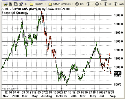
Figure 2: eSIGNAL, SeasonalStrategy. Here is an example of the Soybean_SeasonalStrategy.efs on soybean futures set for a sell month of June (“6”) and buy month of September (“9”).

Figure 3: eSIGNAL, SeasonalStrategyMA. Here is an example of the Soybean_SeasonalStrategyMA.efs on soybean futures configured for a fast moving average of 18 periods and a slow moving average of 120 periods.
The Soybean_SeasonalStrategy.efs formula contains parameters that may be configured through the Edit Studies option to change the buy and sell months. The Soybean_SeasonalStrategyMA.efs formula contains parameters that may be configured through the Edit Studies option to change the fast and slow moving average periods.
To discuss this study or download complete copies of the formula code, please visit the Efs Library Discussion Board forum under the Forums link at www.esignalcentral.com or visit our Efs KnowledgeBase at www.esignalcentral.com/support/kb/efs/. The eSignal formula scripts (Efs) are also available for copying and pasting from the Stocks & Commodities website at Traders.com.
Soybean_SeasonalStrategy.efs
  /*********************************
  Provided By:
  eSignal (Copyright c eSignal), a division of Interactive Data
  Corporation. 2009. All rights reserved. This sample eSignal
  Formula Script (EFS) is for educational purposes only and may be
  modified and saved under a new file name.  eSignal is not responsible
  for the functionality once modified.  eSignal reserves the right
  to modify and overwrite this EFS file with each new release.
Description:
  Soybean Simple Date Seasonal Strategy
Version:            1.0  09/09/2009
Formula Parameters:                         Default:
  SELLMONTH                               6
  BUYMONTH                                9

  Notes:
  The related article is copyrighted material. If you are not a subscriber
  of Stocks & Commodities, please visit www.traders.com.
**********************************/
  var fpArray = new Array();
  var bVersion = null;
function preMain() {
  setPriceStudy(true);
  setShowCursorLabel(false);
  setShowTitleParameters( false );
  setStudyTitle(“Seasonal Strategy”);
  setColorPriceBars(true);
  askForInput();
  var x=0;
  fpArray[x] = new FunctionParameter(“SELLMONTH”, FunctionParameter.NUMBER);
  with(fpArray[x++]){
  setLowerLimit(1);
  setDefault(6);
  }
  fpArray[x] = new FunctionParameter(“BUYMONTH”, FunctionParameter.NUMBER);
  with(fpArray[x++]){
  setLowerLimit(1);
  setDefault(9);
  }
  }
function main(SELLMONTH, BUYMONTH) {
  var nBarState = getBarState();
  var SEASONALBUY = false;
  var SEASONALSHORT = false;
  if (bVersion == null) bVersion = verify();
  if (bVersion == false) return;
  if (getCurrentBarIndex() == 0) return;
  if (nBarState == BARSTATE_ALLBARS) {
  if (SELLMONTH == null) SELLMONTH = 6;
  if (BUYMONTH == null) BUYMONTH = 9;
  }
  setPriceBarColor(Color.black);
  if (getMonth(0) < SELLMONTH  || getMonth(0) > BUYMONTH ) SEASONALBUY = true; else SEASONALBUY = false;
  if (getMonth(0) > SELLMONTH  && getMonth(0) < BUYMONTH + 1) SEASONALSHORT = true; else SEASONALSHORT = false;
  if (SEASONALBUY && !Strategy.isLong()) {
  Strategy.doLong(“Buy”, Strategy.MARKET, Strategy.NEXTBAR);
  }
  if (SEASONALSHORT && !Strategy.isShort()) {
  Strategy.doShort(“Sell”, Strategy.MARKET, Strategy.NEXTBAR);
  }
  if(Strategy.isLong())
  setPriceBarColor(Color.lime);
  if(Strategy.isShort())
  setPriceBarColor(Color.red);
  return;
  }
function verify() {
  var b = false;
  if (getBuildNumber() < 779) {
  drawTextAbsolute(5, 35, “This study requires version 8.0 or later.”,
  Color.white, Color.blue, Text.RELATIVETOBOTTOM|Text.RELATIVETOLEFT|Text.BOLD|Text.LEFT,
  null, 13, “error”);
  drawTextAbsolute(5, 20, “Click HERE to upgrade.@URL=https://www.esignal.com/download/default.asp”,
  Color.white, Color.blue, Text.RELATIVETOBOTTOM|Text.RELATIVETOLEFT|Text.BOLD|Text.LEFT,
  null, 13, “upgrade”);
  return b;
  } else {
  b = true;
  }
  return b;
  }

Soybean_SeasonalStrategyMA.efs
  /*********************************
  Provided By:
  eSignal (Copyright c eSignal), a division of Interactive Data
  Corporation. 2009. All rights reserved. This sample eSignal
  Formula Script (EFS) is for educational purposes only and may be
  modified and saved under a new file name.  eSignal is not responsible
  for the functionality once modified.  eSignal reserves the right
  to modify and overwrite this EFS file with each new release.
Description:
  Simple Moving Average Crossover Soybean Strategy
Version:            1.0  09/09/2009
Formula Parameters:                         Default:
  Fast Length                             18
  Slow Length                             120

  Notes:
  The related article is copyrighted material. If you are not a subscriber
  of Stocks & Commodities, please visit www.traders.com.
**********************************/
  var fpArray = new Array();
  var bInit = false;
  var bVersion = null;
function preMain() {
  setPriceStudy(true);
  setShowCursorLabel(false);
  setShowTitleParameters( false );
  setStudyTitle(“Simple MA Soybean Strategy”);
  setColorPriceBars(true);
  askForInput();
  var x=0;
  fpArray[x] = new FunctionParameter(“FastLength”, FunctionParameter.NUMBER);
  with(fpArray[x++]){
  setName(“Fast Length”);
  setLowerLimit(1);
  setDefault(18);
  }
  fpArray[x] = new FunctionParameter(“SlowLength”, FunctionParameter.NUMBER);
  with(fpArray[x++]){
  setName(“Slow Length”);
  setLowerLimit(1);
  setDefault(120);
  }
  }
var xMAS = null;
  var xMAL = null;
function main(FastLength, SlowLength) {
  var nBarState = getBarState();
  var nMAS = 0;
  var nMAS1 = 0;
  var nMAL = 0;
  var nMAL1 = 0;
  if (bVersion == null) bVersion = verify();
  if (bVersion == false) return;
  if (getCurrentBarIndex() == 0) return;
  if (nBarState == BARSTATE_ALLBARS) {
  if (FastLength == null) FastLength = 18;
  if (SlowLength == null) SlowLength = 120;
  }
  if (bInit == false) {
  xMAS = sma(FastLength);
  xMAL = sma(SlowLength);
  bInit = true;
  }
  setPriceBarColor(Color.black);
  nMAS = xMAS.getValue(0);
  nMAS1 = xMAS.getValue(-1);
  nMAL = xMAL.getValue(0);
  nMAL1 = xMAL.getValue(-1);
  if (nMAL1 == null) return;
  if (nMAS1 < nMAL1 && nMAS > nMAL && !Strategy.isLong())
  Strategy.doLong(“Buy”, Strategy.MARKET, Strategy.NEXTBAR);
  if (nMAS1 > nMAL1 && nMAS < nMAL && !Strategy.isShort())
  Strategy.doShort(“Sell”, Strategy.MARKET, Strategy.NEXTBAR);
  if(Strategy.isLong())
  setPriceBarColor(Color.lime);
  if(Strategy.isShort())
  setPriceBarColor(Color.red);
  return;
  }
function verify() {
  var b = false;
  if (getBuildNumber() < 779) {
  drawTextAbsolute(5, 35, “This study requires version 8.0 or later.”,
  Color.white, Color.blue, Text.RELATIVETOBOTTOM|Text.RELATIVETOLEFT|Text.BOLD|Text.LEFT,
  null, 13, “error”);
  drawTextAbsolute(5, 20, “Click HERE to upgrade.@URL=https://www.esignal.com/download/default.asp”,
  Color.white, Color.blue, Text.RELATIVETOBOTTOM|Text.RELATIVETOLEFT|Text.BOLD|Text.LEFT,
  null, 13, “upgrade”);
  return b;
  } else {
  b = true;
  }
  return b;
  }
![]() WEALTH-LAB: SEASONAL CHANNEL BREAKOUT SYSTEM
WEALTH-LAB: SEASONAL CHANNEL BREAKOUT SYSTEM
The seasonal channel breakout system described by Markos Katsanos in his article in this issue, “A Seasonal System For Trading Soybean Futures,” is quite good at entering near the beginning of new trends, but we occasionally got jiggled out of winning trades prematurely. We found that using a loose chandelier stop as the only exit criteria with an arbitrary Fibonacci period of 55 and an Atr coefficient of 3.0 increased profitability of trading one contract (8.1% vs. 6.7% Apr) and win rate (63.5% vs. 52.1%) while decreasing the number of trades (63 vs. 71) and drawdown (6.13% vs. 6.55% based on $100,000 starting equity). Figure 4 illustrates how the new exit strategy generally helped to keep trades active longer with a well-defined risk.

Figure 4: WEALTH-LAB, seasonal channel breakout system. Our version of the soybean strategy that incorporates the chandelier exit (top) often gave trades the wiggle room they needed for increased profitability, particularly for the trade labeled “3.”
Taking it a step further, applying a 4% risk-stop position sizing strategy more than doubled profit at 16.1% Apr (with a commission of $50 per contract) at the expense of doubling the maximum drawdown to 15.0%, which occurred at the front end of the backtest due to six of eight losing trades (Figure 5). Risk-stop sizing specifies the percentage of portfolio equity that you’re willing to risk on a single trade. Allowing for greater risk — that is, more contracts — magnifies the effect even more.
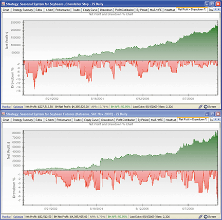
Figure 5: WEALTH-LAB, seasonal channel breakout system. Combining the chandelier exit (top) with a 4% risk stop–sizing strategy more than doubled profit with a well-defined exit (hence, risk).
WealthScript Code (C#):
  /* Seasonal Soybean Strategy with Chandelier exit */
  using System;
  using System.Collections.Generic;
  using System.Text;
  using System.Drawing;
  using WealthLab;
  using WealthLab.Indicators;
  using Community.Components;
namespace WealthLab.Strategies
  {
  public class MyStrategy : WealthScript
  {
 StrategyParameter D1DXY;
  StrategyParameter D2SNL;
  StrategyParameter LRSDXYSELL;
  StrategyParameter LRSNLSELL;
  StrategyParameter chandelierPeriod;
  StrategyParameter chandelierCoeff;
  StrategyParameter chnlLength;
  StrategyParameter doPlot;

  public MyStrategy()
  {
  D1DXY = CreateParameter(“DX LRSlope Period”, 25, 10, 50, 1);
  D2SNL = CreateParameter(“Snl LRSlope Period”, 12, 5, 25, 1);
  LRSDXYSELL = CreateParameter(“DX LRSlope”, 0.3, 0.1, 0.8, 0.1);
  LRSNLSELL = CreateParameter(“Snl LRSlope”, -0.8, -1.2, -0.5, 0.1 );
  chandelierPeriod = CreateParameter(“Chandelier Period”, 55, 8, 89, 1);
  chandelierCoeff = CreateParameter(“Chandelier Coeff”, 3, 1, 5, 0.5);
  chnlLength = CreateParameter(“Channel Period”, 4, 2, 20, 2);
  doPlot = CreateParameter(“Plot All”, 1, 0, 1, 1);
  }
 protected override void Execute()
  {
  // initialization for chandelier stop
  SeriesHelper obj = new SeriesHelper( this );
  double chandelierStop = 0.0;
  int cPer = chandelierPeriod.ValueInt;
  PlotStops();
  HideVolume();

  int buyMonth = 9; int sellMonth = 6;

  // Access external data
  Bars dxy = GetExternalSymbol(“DXY”, true);
  Bars snl = GetExternalSymbol(“SNL”, true);

  // Create and plot indicators
  DataSeries channelHiPlus2 = (Highest.Series(Close, chnlLength.ValueInt) + 2d) >> 1;
  DataSeries channelLoMinus2 = (Lowest.Series(Close, chnlLength.ValueInt) - 2d) >> 1;

  DataSeries dxyLR = LinearReg.Series(dxy.Close, D1DXY.ValueInt);
  DataSeries LRSDXY = ROC.Series( dxyLR, D1DXY.ValueInt ) / D1DXY.ValueInt;
  LRSDXY.Description = “DX Avg ROC(“ + D1DXY.ValueInt + “)”;

  DataSeries snlLR = LinearReg.Series(snl.Close, D2SNL.ValueInt);
  DataSeries LRSNL = ROC.Series(snlLR, D2SNL.ValueInt) / D2SNL.ValueInt;
  LRSNL.Description = “Seasonal Avg ROC(“ + D2SNL.ValueInt + “)”;

  ChartPane slopePane = CreatePane(20, true, true);
  PlotSeries(slopePane, LRSDXY, Color.Black, LineStyle.Solid, 1);
  PlotSeries(slopePane, LRSNL, Color.Green, LineStyle.Histogram, 1);

  if( doPlot.ValueInt == 1 )
  {
  PlotSeries(PricePane, channelHiPlus2, Color.Blue, LineStyle.Dashed, 1);
  PlotSeries(PricePane, channelLoMinus2, Color.Brown, LineStyle.Dashed, 1);
  }

  // Trading Strategy logic
  for(int bar = 3 * GetTradingLoopStartBar(1); bar < Bars.Count; bar++)
  {
  int month = Date[bar].Month;
  bool seasonalBuy = month < sellMonth || month > buyMonth;
  bool seasonalShort = month > sellMonth && month < buyMonth;

  if (IsLastPositionActive)
  {
  Position p = LastPosition;
  // Chandelier stop value using Period: 14, Coefficient: 3
  chandelierStop = obj.ChandelierStop( Bars, bar, p, cPer, chandelierCoeff.Value );
  ExitAtTrailingStop(bar+1, p, chandelierStop);
  }
  else if ( seasonalBuy
  && LRSDXY[bar] < LRSDXYSELL.Value
  && Close[bar] > channelHiPlus2[bar]
  && LRSNL[bar] > LRSNLSELL.ValueInt )
  {
  RiskStopLevel = Close[bar] - 3d * ATR.Series(Bars, cPer)[bar];
  BuyAtMarket(bar + 1);
  }
  else if (seasonalShort
  && LRSDXY[bar] > -LRSDXYSELL.Value
  && Close[bar] < channelLoMinus2[bar]
  && LRSNL[bar] < -LRSNLSELL.ValueInt )
  {
  RiskStopLevel = Close[bar] + 3d * ATR.Series(Bars, cPer)[bar];
  ShortAtMarket(bar + 1);
  }
  }
  }
  }
  }
![]() AMIBROKER: SEASONAL CHANNEL BREAKOUT SYSTEM
AMIBROKER: SEASONAL CHANNEL BREAKOUT SYSTEM
In “A Seasonal System For Trading Soybean Futures” in this issue, author Markos Katsanos presents a trading system that combines intermarket data, seasonal factors, and price action.
Coding such an indicator is relatively straightforward. A ready-to-use formula is presented in Listing 1. To use it, enter the formula in the Afl Editor, then select “Send to automatic analysis.” Note that you would need to adjust the symbol names for the dollar index and seasonal data to match your data source symbology. In the Automatic Analysis Settings window, you should also set trading delays to “1” and trade prices to “open price.”
LISTING 1
  Length = 4;
  d1dxy = 25;
  d2snl = 12;
  Sellmonth = 6;
  Buymonth = 9;
  Lrsnlsell = -0.8;
  Lrsdxysell = 0.3;
  MAsnl = 15;
  MAsell = 15;
  MAdxy = 50;
data2 = Foreign(„DollarIndex”, „C”);
  data3 = Foreign(„SeasonalData”, „C”);
RS = EMA( C/data3, 3 );
LRSNL = 100 * LinRegSlope( RS, D2SNL )/LinearReg( RS, D2SNL );
  LRSDXY = 100 * LinRegSlope( data2, D1DXY )/LinearReg( data2, D1DXY );
SeasonalBuy = Month() < SellMonth OR Month() > BuyMonth;
  SeasonalShort = Month() > SellMonth AND Month() < BuyMonth+1;
Buy = SeasonalBuy AND
  LRSDXY < LRSDXYSELL AND
  C > HHV( Ref( C, -1 ), Length ) + 2 AND
  LRSNL > LRSNLSell;

easonalShort AND
  C < LLV( Ref( C, -1 ), Length ) - 2 AND
  LRSDXY > - LRSDXYSELL AND
  LRSNL < -LRSNLSELL;

Sell1 = C < EMA( C, MASELL ) AND
  LRSNL < LRSNLSELL;
Sell2 = C < EMA( C, MASELL ) AND
  ROC( EMA( data2, MADXY ), 1 ) > 0 AND
  LRSDXY > LRSDXYSELL;
Sell = Sell1 OR Sell2;
Cover1 = C > EMA( C, MASELL ) AND
  LRSNL > - LRSNLSELL;
Cover2 = C > EMA( C, MASELL ) AND
  ROC( EMA( data2, MADXY ), 1 ) < 0 AND
  data3 > EMA( data3, MASNL );
Cover = Cover1 OR Cover2;
Plot( LRSNL, „LRSNL”, colorRed );
  Plot( LRSDXY , „LRSDXY „, colorBlue );
![]() NEUROSHELL TRADER: SEASONAL CHANNEL BREAKOUT SYSTEM
NEUROSHELL TRADER: SEASONAL CHANNEL BREAKOUT SYSTEM
Markos Katsanos’s system for trading soybean futures described in his article in this issue can be easily implemented in NeuroShell Trader (Figure 6) by combining a few of NeuroShell Trader’s 800+ indicators. First, select “New Indicator …” from the Insert menu and use the Indicator Wizard to create the following indicator:
RS:
  ExpAvg( Divide( Close, Seasonal Data Close ), 3 )
LRSNL:
  Multiply2 (Divide ( Divide ( Subtract ( LinTimeRegPredValue(RS, 12, 12), LinTimeRegPredValue(RS, 12, 0) ), LinTimeRegPredValue(RS, 12, 12) ), 12 ), 100 )
LRSDXY:
  Multiply2 (Divide ( Divide ( Subtract ( LinTimeRegPredValue(Dollar Index Close, 25, 25), LinTimeRegPredValue(Dollar Index Close, 25, 0) ), LinTimeRegPredValue(Dollar Index Close, 25, 25) ), 25 ), 100 )
SEASONALBUY:
  Or2( A<B( MonthOfYear(Date), 6), A>B(MonthOfYear (Date), 9 )
SEASONALSHORT:
  And2( A>B(MonthOfYear (Date), 6), A<B(MonthOfYear (Date), Add2( 9, 1) ) )
CHANNELBUY
  A>B ( Close, Add2( Max( Lag( Close, 1), 4), 2) )
CHANNELSHORT
  A<B ( Close, Subtract( Min( Lag( Close, 1), 4), 2) )
Then, to set up Katsanos’ soybean futures seasonal trading system, select “New Trading Strategy …” from the Insert menu and enter the following in the appropriate locations of the Trading Strategy Wizard:
Long Entry when all of the following conditions are true:
  And4 ( SEASONALBUY, A<B( LRSDXY, 0.3 ), CHANNELBUY, A>B( LRSNL, -0.8 )
  Long Exit when ONE of the following conditions are true:
  AND2 ( A<B( Close, ExpAvg( Close, 15 ), A<B ( LRSNL, -0.8 ) )
  AND3 ( A<B( Close, ExpAvg( Close, 15 ) ), A>B( Momentum( ExpAvg( Dollar Index Close, 50 ), 1), 0), A>B( LRSDXY, 0.3 ) )
Short Entry when all of the following conditions are true:
  And4 ( SEASONALSHORT, CHANNELSHORT , A>B( LRSDXY, -0.3 ), A<B( LRSNL, 0.8 )
Short Exit when ONE of the following conditions are true:
  AND2 ( A>B ( Close, ExpAvg(Close, 15) ), A>B ( LRSNL, 0.8 ) )
  AND3 ( A>B ( Close, ExpAvg(Close, 15) ), A<B( Momentum( ExpAvg( Dollar Index Close, 50 ), 1), 0), A>B (Seasonal Data Close, ExpAvg (Seasonal Data Close, 15 ) )
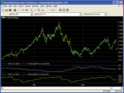
Figure 6: NEUROSHELL TRADER, Seasonal System for trading Soybean Futures
If you have NeuroShell Trader Professional, you can also choose whether the system parameters should be optimized. After backtesting the trading strategy, use the “Detailed Analysis …” button to view the backtest and trade-by-trade statistics for the system.
![]() AIQ: SEASONAL CHANNEL BREAKOUT SYSTEM
AIQ: SEASONAL CHANNEL BREAKOUT SYSTEM
This Aiq code is based on Markos Katsanos’ article in this issue, “A Seasonal System For Trading Soybean Futures.”
All three systems that Katsanos describes in his article are included in one Eds file named “SoySeas.eds.” Since the author supplied all three of the data files used by the systems with his article, I imported the files into the Aiq database using the Data Transfer Utility (Dtu). These data files in the Aiq format will be available at my website for download. In addition, I put the one ticker that is traded, ZS_KAT.dta, on a list by itself. The list can also be downloaded with the Eds file. All of these files will be zipped into one file for download. Once you have downloaded the zipped file to a temporary directory and unzipped it to a second temporary directory, copy the files to the following locations:
- *.dta files to c:\Wintes32\Tdata\
- *.eds file to c:\Wintes32\EDS Strategies\
- *.lis file to c:\Wintes32\
After copying the files to these directories, run the “rebuild master ticker list” from the “utilities” dropdown menu within the data manager. Now you are ready to open and run the Eds file.
The code can be downloaded from the Aiq website at www.aiqsystems.com and also from www.TradersEdgeSystems.com/traderstips.htm. (Note: To download, right-click on the .eds link, then save-as.)
! SOYBEAN SEASONAL SYSTEMS
  ! Author: Markos Katsanos, TASC November 2009
  ! Coded by: Richard Denning 9/12/09
  ! www.TradersEdgeSystems.com
! INPUTS:
  LENGTH		is 4.
  D1DXY 		is 25.
  D2SNL 		is 12.
  SELLMN 		is 6.
  BUYMN		is 9.
  LRSNLSELL	is -0.8.
  LRSDXYSELL	is 0.3.
  MASNL		is 15.
  MASELL		is 15.
  MADXY		is 50.
  FASTLENGTH	is 18.
  SLOWLENGTH	is 120.
! INDICATORS & UDFs USED FOR THE SYSTEMS:
  C		is [close].		  ! ZS_KAT.dta
  dollarIdx	is tickerUDF(“DXY_KAT”,C).! Authors data file
  seasData	is tickerUDF(“SNL_KAT”,C).! Authors data file
  HD		is hasdatafor(125).
RS		is expavg(C / seasData,3).
  b_rs  		is slope2(RS,D2SNL).
  intercept_rs  	is sum(RS,D2SNL)/D2SNL - (b_rs*(D2SNL+1)/2).
  rsLRV  		is intercept_rs + (D2SNL-1)*b_rs.
  rsLRVd2 	is intercept_rs + (D2SNL-1-D2SNL)*b_rs.
  LrsNL 		is (rsLRV / rsLRVd2 -1) / D2SNL * 100.

  b_dlr  		is slope2(dollarIdx,D1DXY).
  intercept_dlr  	is sum(dollarIdx,D1DXY)/D1DXY-(b_dlr*(D1DXY+1)/2).
  dlrLRV  	is intercept_dlr + (D1DXY-1)*b_dlr.
  dlrLRVd1 	is intercept_dlr + (D1DXY-1-D1DXY)*b_dlr.
  LrsDxy 		is (dlrLRV / dlrLRVd1 -1) / D1DXY * 100.
! USE THE FOLLOWING RULES FOR THE SIMPLE SEASONAL
  ! Note: they are also part of the Seasonal with Channel Breakout
  month		is month().
  seasonalBuy	if month() < SELLMN or month() > BUYMN.
  seasonalShort	if month() > SELLMN and month() < BUYMN+1.
! USE “BUY/EXITLONG” & “SHORT/EXITSHORT” FOR THE SEASONAL
  ! WITH CHANNEL BREAKOUT SYSTEM:
  HC		is highresult(C,LENGTH,1) + 2.
Buy		if seasonalBuy and LrsDxy < LRSDXYSELL
  and C > HC and LrsNL > LRSNLSELL and HD > 51.
ExitLong	if ( C < expavg(C,MASELL) and LrsNL < LRSNLSELL )
  or ( C < expavg(C,MASELL)
  and expavg(dollarIdx,MADXY)>expavg(dollarIdx,MADXY,1)
  and LrsDxy > LRSDXYSELL )
  or Short.
Short		if seasonalShort and C < lowresult(C,LENGTH,1) - 2
  and LrsDxy > -LRSDXYSELL and LrsNL < -LRSNLSELL
  and HD > 51.
ExitShort if ( C > expavg(C,MASELL) and LrsNL > -LRSNLSELL )
  or ( C > expavg(C,MASELL)
  and expavg(dollarIdx,MADXY)<expavg(dollarIdx,MADXY,1)
  and seasData > expavg(seasData,MASNL) )
  or Buy.
! USE THE FOLLOWING FOR THE SIMPLE MOVING AVERAGE CROSS OVER:
  MAS		is simpleavg(C,FASTLENGTH).
  MAL		is simpleavg(C,SLOWLENGTH).
buyXUP		if MAS > MAL and valrule(MAS < MAL,1) and HD > 120.
  sellXDN		if MAS < MAL and valrule(MAS > MAL,1) and HD > 120.
![]() TRADERSSTUDIO: SEASONAL CHANNEL BREAKOUT SYSTEM
TRADERSSTUDIO: SEASONAL CHANNEL BREAKOUT SYSTEM
The TradersStudio code for the soybean trading system from the article, “A Seasonal System For Trading Soybean Futures” by Markos Katsanos in this issue, together with the code for the simple seasonal system and the simple moving average crossover system, is provided below and is also available for download from the following websites:
TradersStudio website:
www.TradersStudio.com ⇒Traders Resources ⇒FreeCode
TradersEdgeSystems website:
www.TradersEdgeSystems.com/traderstips.htm
The code is also available at the Traders.com website:
www.Traders.com ⇒Stocks & Commodities ⇒Current Issue ⇒Traders’ Tips
In reviewing Katsanos’ system, I was struck by the extraordinarily high returns. In reviewing how the seasonal system was developed, I noticed it was developed with the same data over which the system was tested, and this appears to me to create a strong look-ahead bias. To avoid this issue, we should develop the seasonal system on data that comes before the first date on which we want to test the system. In order to do this, we need to use all of the soybean cash index data that goes back to June 1969 (data from Pinnacle). We can use several methods to get a seasonal analysis, and then we need to decide whether we will use a rolling window or an anchored window. If there is seasonal drift, it would be better to use the rolling window approach, since the anchored window will be slow to react to changes in the seasonal due to fundamental changes in the markets, such as a shift to higher production in the southern hemisphere, which has the opposite growing season than the US, and would tend to nullify the effect of the seasonal.
TradersStudio has an add-in module called the Universal Seasonal that does extensive seasonal analysis and allows you to calculate a walkforward seasonal on any market. It does not require using the related cash indexes, since the seasonal system does not use the raw price data but rather looks at normalized rates of change. The Universal Seasonal add-in module includes 12 indicators, 20 functions, and one example trading system that allows extensive seasonal research to be done without any look-ahead bias. In Figure 7, two of the most useful indicators and functions are shown on a chart of soybean futures (data from Pinnacle, symbol S_Rev). The first panel in Figure 7 (underneath the soybean futures chart) is the RuggieroBarna seasonal index, which is calculated as follows:
- For each trading day of the year, record the “next n-day” returns and the percentage of time the market moved up (for positive returns) and down (for negative returns).
- Multiply this n-day return by the proper percentage.
- Scale the numbers calculated in step 2 between 1 and -1 over the trading year.
In the second panel of Figure 7 is the SeasonalCorrel indicator, which shows the correlations of current market data to the seasonal historical data. It uses the Spearman rank correlation function. In developing a seasonal trading system, we may want to reverse the trade logic when the current conditions are negatively correlated to the seasonality, or in any case, to filter out signals when correlation is low. With both indicators, for the “n-day return” and “n-day correlation,” n was set to 20 and a rolling window of 12 years of data was used to develop the seasonal for each day of the year.
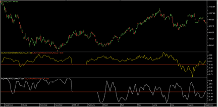
Figure 7: TRADERSSTUDIO. Here is a one-year chart of soybean futures with the RuggieroBarna seasonal indicator and the SeasonalCorrel indicator.
TradesStudio code:
  Sub SOYBEAN_SEAS_CHAN_BO(LENGTH,D1DXY,D2SNL,SELLMONTH,BUYMONTH,LRSNLSELL,LRSDXYSELL,MASNL,MASELL,MADXY)
  ‘LENGTH(4), D1DXY(25), D2SNL(12), SELLMONTH(6), BUYMONTH(9), LRSNLSELL(-.8), LRSDXYSELL(.3), MASNL(15), MASELL(15), MADXY(50)
  Dim rs As BarArray
  Dim rsLR As BarArray
  Dim rsLR_D2 As BarArray
  Dim LrsNL As BarArray
  Dim S2 As BarArray
  Dim StopL As BarArray
  Dim SeasonalBuy As BarArray
  Dim SeasonalShort As BarArray
  Dim LrsDxy As BarArray
  Dim dxyLR As BarArray
  Dim dxyLR_D1 As BarArray
  Dim Seasonal As BarArray
  Dim DollarIndx As BarArray
 If BarNumber=FirstBar Then
  rs = 0
  LrsNL = 0
  S2 = 0
  StopL = 0
  SeasonalBuy = False
  SeasonalShort = False
  LrsDxy = 0
  End If

  DollarIndx = C Of Independent1
  Seasonal = C Of Independent2

  Dim tempRS As BarArray
  If Seasonal > 0 Then
  tempRS = C/Seasonal
  End If

  If CurrentBar - 1 > 3 Then
  rs = XAverage(tempRS,3,0)
  End If
  If CurrentBar - 1 > D2SNL+3 Then
  rsLR = LR_VAL(rs,D2SNL,0)
  rsLR_D2 = LR_VAL(rs,D2SNL,D2SNL)
  If rsLR_D2 <> 0 And D2SNL <> 0 And rs <> 0 Then
  LrsNL = (rsLR / rsLR_D2 - 1) / D2SNL*100
  ‘Print FormatDateTime(Date),” rs “, Round(rs,4), “ rsLR “,Round(rsLR,4),  “ rsLR_D2 “, Round(rsLR_D2,4),” LrsNL “,Round(LrsNL,4),
  End If
  End If
  If CurrentBar - 1 > D1DXY+3 Then
  dxyLR = LR_VAL(DollarIndx,D1DXY,0)
  dxyLR_D1 = LR_VAL(DollarIndx,D1DXY,D1DXY)
  If dxyLR_D1 <> 0  And D1DXY <> 0 And rs <> 0 Then
  LrsDxy = (dxyLR/dxyLR_D1-1) / D1DXY*100
  ‘Print FormatDateTime(Date),” $idx “, Round(DollarIndx,2), “ dxyLR “,Round(dxyLR,4),  “ dxyLR_D1 “, Round(dxyLR_D1,4),” LrsDxy “,Round(LrsDxy,4),
  End If
  End If
  SeasonalBuy = Month(D) < SELLMONTH Or Month(D) > BUYMONTH
  SeasonalShort = Month(D) > SELLMONTH And Month(D) < BUYMONTH+1

  ‘Long and Short Entry Conditions-------
  If SeasonalBuy And LrsDxy < LRSDXYSELL And C > (Highest(C[1],LENGTH,0)+2) And LrsNL > LRSNLSELL Then
  Buy(“LE”,1,0,Market,Day)
  ‘Print FormatDateTime(Date),” LrsNL “, Round(LrsNL,4),” LRSDXYSELL “,LRSDXYSELL, “ LRSNLSELL “ ,LRSNLSELL,” LrsDxy “,Round(LrsDxy,4), “ C “,C,” HC “, Round(Highest(C[1],LENGTH,0)+2,4)
  End If
  If SeasonalShort And C < Lowest(C,LENGTH,1) - 2 And LrsDxy > -LRSDXYSELL And LrsNL < -LRSNLSELL Then
  Sell(“SE”,1,0,Market,Day)
  End If
‘Exit conditions
  ‘RS with SNL Exit
  If C < XAverage(C,MASELL,0)And LrsNL < LRSNLSELL Then
  ExitLong(“LX RS”,””,1,0,Market, Day)
  End If
  If C < XAverage(C,MASELL,0)And XAverage(DollarIndx,MADXY,0)> XAverage(DollarIndx,MADXY,1) And LrsDxy > LRSDXYSELL Then
  ExitLong(“LX DXY”,””,1,0,Market,Day)
  End If

  ‘RS with SNL Exit
  If C > XAverage(C,MASELL,0)And LrsNL > -LRSNLSELL Then
  ExitShort(“SX RS”,””,1,0,Market,Day)
  End If
  If C > XAverage(C,MASELL,0)And XAverage(DollarIndx,MADXY,0)< XAverage(DollarIndx,MADXY,1) And Seasonal > XAverage(Seasonal,MASNL, 0) Then
  ExitShort(“SX DXY”,””,1,0,Market,Day)
  End If
  End Sub
  ‘_______END SEASONAL SYSTEM WITH CHANNEL BREAKOUT__________
‘LINEAR REGRESSION END POINT VALUE
  ‘Coded by: Richard Dennning 1/21/08
Function LR_VAL(price As BarArray, LRlen, TargetB) As BarArray
  Dim rSqrd,slopeR As Double
  Dim endVal As BarArray
  LR_VAL = LR_SRV(price, LRlen, TargetB, rSqrd, slopeR, endVal)
  End Function
  ‘_______END LR END POINT FUNCTION__________________
‘ LINEAR REGRESSION FUNCTION
  ‘ Coded by Richard Denning 01/21/08
‘Parameters
‘Y  specifies which price of the asset of interest is To be used
  ‘SLen the number Of trailing bars To consider
  ‘TargetB represents the number Of bars into the future Or back into the past
  ‘Returns a numeric value containing the current value Of the specified regression line at TargetB.
  ‘Changes values of variables rSqrd, slopeR, endVal to those the least squares line computed by the function
  ‘ R squared (rSqrd) is the measure of how well the line fits the data (will vary from 0 (no fit) to 1.00 (perfect fit)
  ‘ slope (slopeR) is the risk ove run of the line
  ‘ endVal is the value of the line at the current bar
‘the regression formulas can be checked using the Excel tutorial on linear regression found at:
  ‘https://phoenix.phys.clemson.edu/tutorials/excel/regression.html
Function LR_SRV(Y As BarArray, SLen, TargetB, ByRef rSqrd, ByRef slopeR, ByRef endVal) as bararray
  Dim X, sumX, sumSqrX, sumY, sumSqrY, sumXY, numer, denom1, denom2 As Double
  Dim Slope As Double
  Dim Intercept As Double
  Dim R As Double
  Dim myDate As String
  myDate = FormatDateTime(Date)

  If SLen <= 0 Then
  LR_SRV = 0
  Else
  sumX = 0
  sumSqrX = 0
  sumY = 0
  sumSqrY = 0
  sumXY = 0

  For X = 0 To SLen - 1
  sumX = sumX + X+1
  sumSqrX = sumSqrX + (X+1)*(X+1)
  sumY = sumY + Y[X]
  sumSqrY = sumSqrY + Y[X] * Y[X]
  sumXY = sumXY + (X+1) * Y[SLen-X-1]
  Next

  numer = (SLen * sumXY - sumX * sumY)

  ‘slope
  denom1 = (SLen * sumSqrX - sumX * sumX)
  If denom1 <> 0 Then
  Slope = numer / denom1
  Else
  Slope = 0
  End If
  slopeR = Slope

  ‘intercept
  if slen <> 0 then Intercept = (sumY - Slope * sumX) / SLen

  ‘R squared
  denom2 = (Sqr( (SLen * sumSqrX - sumX*sumX)*(SLen * sumSqrY - (sumY * sumY)) ))
  If denom2 <> 0 Then
  R = numer / denom2
  rSqrd = R * R
  Else
  rSqrd = 0
  End If

  ‘end value of linear regression line
  endVal = Intercept + Slope * (SLen)

  ‘projected value of linear regression line at target bar
  LR_SRV = Intercept + Slope * (SLen - 1 - TargetB)

  ‘Print “Date: “, myDate, “ sumX: “, sumX,  “ sumY: “, sumY, “ sumXY: “, sumXY, “ sumXsqrd: “, sumSqrX, “ sumYsqrd: “, sumSqrY, “ R Sqr: “, rSqrd, “ Slope: “, slopeR, “ Intercept: “, Intercept

  End If
  End Function
  ‘________________END LR MULTI-OUTPUT FUNCTION__________________
Sub SOY_SIMPLE_SEAS(SELLMONTH, BUYMONTH)
  ‘SELLMONTH = 6,’BUYMONTH = 9
  Dim SeasonalBuy As Boolean
  Dim SeasonalShort As Boolean
  If BarNumber=FirstBar Then
  SeasonalBuy = False
  SeasonalShort = False
  End If
  SeasonalBuy = Month(D) < SELLMONTH Or Month(D) > BUYMONTH
  SeasonalShort = Month(D) > SELLMONTH And Month(D) < BUYMONTH + 1
  If SeasonalBuy Then
  Buy(“LE”, 1, 0, Close, Day)
  End If
  If SeasonalShort Then
  Sell(“SE”, 1, 0, Close, Day)
  End If
  End Sub
  ‘_______________END SIMPLE SEASONAL SYSTEM_____________________
Sub SOY_SIMPLE_MA_XO(FASTLENGTH, SLOWLENGTH)
  ‘FASTLENGTH = 18,’SLOWLENGTH = 120
  Dim MAS As BarArray
  Dim MAL As BarArray
  If BarNumber = FirstBar Then
  MAS = 0
  MAL = 0
  End If
  MAS = Average(C, FASTLENGTH)
  MAL = Average(C, SLOWLENGTH)
  If CrossesOver(MAS, MAL) Then
  Buy(“LE_MAcross”, 1, 0, Market, Day)
  End If
  If CrossesUnder(MAS, MAL) Then
  Sell(“SE_MAcross”, 1, 0, Market, Day)
  End If
  End Sub
  ‘______________END SIMPLE MA CROSS-OVER SYSTEM___________________
![]() TRADECISION: SEASONAL CHANNEL BREAKOUT SYSTEM
TRADECISION: SEASONAL CHANNEL BREAKOUT SYSTEM
The article by Markos Katsanos in this issue, “A Seasonal System For Trading Soybean Futures,” demonstrates the correlation between the soybean historical average seasonal prices and the dollar index to develop a trading system that exploits historical seasonal patterns to trade soybean futures (Figure 8).
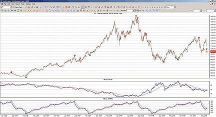
FIGURE 8: TRADECISION, SEASONAL CHANNEL STRATEGY SIGNALS. Buy and sell signals generated by the seasonal channel strategy are superimposed in red and green, respectively, and exit signals are not filled. The dollar index is plotted in the middle window with the historical average seasonal prices below that.
You can recreate the soybean seasonal channel breakout strategy using Tradecision’s Strategy Builder. Here are the strategy rules:
Entry Long:
{LENGTH=Channel length in days,
  D1DXY=Days for the Dollar Index linear regression slope calculation
  D2SNL=Days for the Seasonal data linear regression slope calculation
  LRSNLSELL= Seasonal data linear regression slope per day
  LRSDXYSELL=Dollar index linear regression slope per day
  MASNL=Days for the seasonal exponential moving average sell/buytocover conditions
  MASELL=Days for the Soybean exponential moving average sell/buytocover conditions
  MADXY=Days for the Dollar Index moving average sell/buytocover conditions}
 VARIABLES
  LENGTH:=4;
  D1DXY:=25;
  D2SNL:=12;
  SELLMONTH:=6;
  BUYMONTH:=9;
  LRSNLSELL:=-0.8;
  LRSDXYSELL:=0.3;
  MASNL:=15;
  MASELL:=15;
  MADXY:=50;
  RS:=0;
  LRSNL:=0;
  S2:=0;
  STOPL:=0;
  SEASONALBUY:=FALSE;
  SEASONALSHORT:=FALSE;
  LRSDXY:=0;
  END_VARIABLES
 IF BARNUMBER>3 THEN BEGIN
  RS:=EMA((Close / External(«Close»,»SNL»)), 3);
  END;
  IF BARNUMBER >D2SNL + 3 THEN BEGIN
  LRSNL:=(LRL(RS, D2SNL, 0) - LRL(RS, D2SNL, D2SNL)) / LRL(RS, D2SNL, D2SNL) / D2SNL * 100;
  END;
  IF BARNUMBER >D1DXY THEN BEGIN
  LRSDXY:=(LRL(External(«Close»,»DXY»),D1DXY,0) - LRL(External(«Close»,»DXY»),D1DXY,D1DXY)) /
  LRL(External(«Close»,»DXY»),D1DXY,D1DXY) / D1DXY * 100;
  END;
 SEASONALBUY:= Month < SELLMONTH OR Month > BUYMONTH;
  SEASONALSHORT:= Month > SELLMONTH AND Month < BUYMONTH+1;
 {Buy condition}
  IF SEASONALBUY AND LRSDXY < LRSDXYSELL AND C > (HIGHEST(Close\1\,LENGTH)+2) AND LRSNL > LRSNLSELL THEN return TRUE;
  return FALSE;
Exit Long:
{LENGTH=Channel length in days,
  D1DXY=Days for the Dollar Index linear regression slope calculation
  D2SNL=Days for the Seasonal data linear regression slope calculation
  LRSNLSELL= Seasonal data linear regression slope per day
  LRSDXYSELL=Dollar index linear regression slope per day
  MASNL=Days for the seasonal exponential moving average sell/buytocover conditions
  MASELL=Days for the Soybean exponential moving average sell/buytocover conditions
  MADXY=Days for the Dollar Index moving average sell/buytocover conditions}
 VARIABLES
  LENGTH:=4;
  D1DXY:=25;
  D2SNL:=12;
  SELLMONTH:=6;
  BUYMONTH:=9;
  LRSNLSELL:=-0.8;
  LRSDXYSELL:=0.3;
  MASNL:=15;
  MASELL:=15;
  MADXY:=50;
  RS:=0;
  LRSNL:=0;
  S2:=0;
  STOPL:=0;
  SEASONALBUY:=FALSE;
  SEASONALSHORT:=FALSE;
  LRSDXY:=0;
  END_VARIABLES
 IF BARNUMBER>3 THEN BEGIN
  RS:=EMA((Close / External(«Close»,»SNL»)), 3);
  END;
  IF BARNUMBER >D2SNL + 3 THEN BEGIN
  LRSNL:=(LRL(RS, D2SNL, 0) - LRL(RS, D2SNL, D2SNL)) / LRL(RS, D2SNL, D2SNL) / D2SNL * 100;
  END;
  IF BARNUMBER >D1DXY THEN BEGIN
  LRSDXY:=(LRL(External(«Close»,»DXY»),D1DXY,0) - LRL(External(«Close»,»DXY»),D1DXY,D1DXY)) /
  LRL(External(«Close»,»DXY»),D1DXY,D1DXY) / D1DXY * 100;
  END;
 SEASONALBUY:= Month < SELLMONTH OR Month > BUYMONTH;
  SEASONALSHORT:= Month > SELLMONTH AND Month < BUYMONTH+1;
 IF {IsLongPosition() AND }BarsSinceEntry > 1 THEN BEGIN
  IF Close < EMA(Close, MASELL) AND LRSNL < LRSNLSELL THEN
  return TRUE;
  IF Close < EMA(Close, MASELL) AND EMA(External(«Close»,»DXY»),MADXY) > EMA(External(«Close»,»DXY»),MADXY)\1\
  AND LRSDXY>LRSDXYSELL THEN
  return TRUE;
  END;
  return FALSE;
Entry Short:
{LENGTH=Channel length in days,
  D1DXY=Days for the Dollar Index linear regression slope calculation
  D2SNL=Days for the Seasonal data linear regression slope calculation
  LRSNLSELL= Seasonal data linear regression slope per day
  LRSDXYSELL=Dollar index linear regression slope per day
  MASNL=Days for the seasonal exponential moving average sell/buytocover conditions
  MASELL=Days for the Soybean exponential moving average sell/buytocover conditions
  MADXY=Days for the Dollar Index moving average sell/buytocover conditions}
 VARIABLES
  LENGTH:=4;
  D1DXY:=25;
  D2SNL:=12;
  SELLMONTH:=6;
  BUYMONTH:=9;
  LRSNLSELL:=-0.8;
  LRSDXYSELL:=0.3;
  MASNL:=15;
  MASELL:=15;
  MADXY:=50;
  RS:=0;
  LRSNL:=0;
  S2:=0;
  STOPL:=0;
  SEASONALBUY:=FALSE;
  SEASONALSHORT:=FALSE;
  LRSDXY:=0;
  END_VARIABLES
 IF BARNUMBER>3 THEN BEGIN
  RS:=EMA((Close / External(«Close»,»SNL»)), 3);
  END;
  IF BARNUMBER >D2SNL + 3 THEN BEGIN
  LRSNL:=(LRL(RS, D2SNL, 0) - LRL(RS, D2SNL, D2SNL)) / LRL(RS, D2SNL, D2SNL) / D2SNL * 100;
  END;
  IF BARNUMBER >D1DXY THEN BEGIN
  LRSDXY:=(LRL(External(«Close»,»DXY»),D1DXY,0) - LRL(External(«Close»,»DXY»),D1DXY,D1DXY)) /
  LRL(External(«Close»,»DXY»),D1DXY,D1DXY) / D1DXY * 100;
  END;
 SEASONALBUY:= Month < SELLMONTH OR Month > BUYMONTH;
  SEASONALSHORT:= Month > SELLMONTH AND Month < BUYMONTH+1;
 {Sell condition}
  IF SEASONALSHORT AND C < LOWEST(C,LENGTH)\1\ - 2 AND LRSDXY > -LRSDXYSELL
  AND LRSNL < -LRSNLSELL THEN
  return TRUE;
  return FALSE;
Exit Short:
{LENGTH=Channel length in days,
  D1DXY=Days for the Dollar Index linear regression slope calculation
  D2SNL=Days for the Seasonal data linear regression slope calculation
  LRSNLSELL= Seasonal data linear regression slope per day
  LRSDXYSELL=Dollar index linear regression slope per day
  MASNL=Days for the seasonal exponential moving average sell/buytocover conditions
  MASELL=Days for the Soybean exponential moving average sell/buytocover conditions
  MADXY=Days for the Dollar Index moving average sell/buytocover conditions}
 VARIABLES
  LENGTH:=4;
  D1DXY:=25;
  D2SNL:=12;
  SELLMONTH:=6;
  BUYMONTH:=9;
  LRSNLSELL:=-0.8;
  LRSDXYSELL:=0.3;
  MASNL:=15;
  MASELL:=15;
  MADXY:=50;
  RS:=0;
  LRSNL:=0;
  S2:=0;
  STOPL:=0;
  SEASONALBUY:=FALSE;
  SEASONALSHORT:=FALSE;
  LRSDXY:=0;
  END_VARIABLES
 IF BARNUMBER>3 THEN BEGIN
  RS:=EMA((Close / External(«Close»,»SNL»)), 3);
  END;
  IF BARNUMBER >D2SNL + 3 THEN BEGIN
  LRSNL:=(LRL(RS, D2SNL, 0) - LRL(RS, D2SNL, D2SNL)) / LRL(RS, D2SNL, D2SNL) / D2SNL * 100;
  END;
  IF BARNUMBER >D1DXY THEN BEGIN
  LRSDXY:=(LRL(External(«Close»,»DXY»),D1DXY,0) - LRL(External(«Close»,»DXY»),D1DXY,D1DXY)) /
  LRL(External(«Close»,»DXY»),D1DXY,D1DXY) / D1DXY * 100;
  END;
 SEASONALBUY:= Month < SELLMONTH OR Month > BUYMONTH;
  SEASONALSHORT:= Month > SELLMONTH AND Month < BUYMONTH+1;
 IF BarsSinceEntry > 1 THEN BEGIN
  IF Close > EMA(Close, MASELL) AND LRSNL > -LRSNLSELL THEN
  return TRUE;
  IF Close > EMA(Close, MASELL) AND EMA(External(«Close»,»DXY»),MADXY) < EMA(External(«Close»,»DXY»),MADXY)\1\
  AND External(«Close»,»SNL») > EMA(External(«Close»,»SNL»),MASNL) THEN
  return TRUE;
  END;
  return FALSE;
Next, create the soybean simple date seasonal strategy:
Entry Long:
VARIABLES
  SELLMONTH:=6;
  BUYMONTH:=9;
  SEASONALBUY:= FALSE;
  END_VARIABLES
SEASONALBUY:= Month < SELLMONTH OR Month > BUYMONTH;
IF SEASONALBUY THEN return TRUE;
  return FALSE;
Entry Short:
VARIABLES
  SELLMONTH:=6;
  BUYMONTH:=9;
  SEASONALSHORT:=FALSE;
  END_VARIABLES
SEASONALSHORT:= MONTH > SELLMONTH AND MONTH < BUYMONTH+1;
IF SEASONALSHORT THEN return TRUE;
  return FALSE;
Finally, create the simple moving average crossover strategy:
Entry Long:
VARIABLES
  FastLength:=18;
  SlowLength:=120;
  MAS:=0;
  MAL:=0;
  AverageFC:=0;
  End_var
MAS:= AverageFC( C, FastLength ) ;
  MAL:= AverageFC( C, SlowLength ) ;
IF BarNumber > SLOWLENGTH THEN BEGIN
  IF CrossAbove(MAS,MAL) THEN return TRUE;
  END;
  return FALSE;
Entry Short:
VARIABLES
  FastLength:=18;
  SlowLength:=120;
  MAS:=0;
  MAL:=0;
  AverageFC:=0;
  End_var
MAS:= AverageFC( C, FastLength ) ;
  MAL:= AverageFC( C, SlowLength ) ;
IF BarNumber > SLOWLENGTH THEN BEGIN
  IF CrossBelow(MAS,MAL) THEN return TRUE;
  END;
  return FALSE;
In addition, create the AverageFC function using Tradecision's Function Builder:
  function (Price:NUMERIC=C, Length:NUMERIC=18):Numeric;
  return CumSum( Price, Length ) / Length;
To import the strategy into Tradecision, visit the area “Traders’ Tips from TASC Magazine” at www.tradecision.com/support/tasc_tips/tasc_traders_tips.htm or copy the code from the Stocks & Commodities website at www.traders.com.
![]() TRADE NAVIGATOR: SEASONAL CHANNEL BREAKOUT SYSTEM
TRADE NAVIGATOR: SEASONAL CHANNEL BREAKOUT SYSTEM
Here, we will show you how to recreate the strategies from Markos Katsanos’ article in this issue, “A Seasonal System For Trading Soybean Futures.” These strategies will require the Platinum version of Trade Navigator as well as the Advanced Seasonal Cycles Library.
The strategy for this article is easy to recreate and test in Trade Navigator. First, you will need to set up some functions to be used in the strategies, as follows.
Go to the Functions tab in the Trader’s Toolbox and click on the New button. Type in the following code:
Close Of “dx-067”
Click the Save button, type “DX” for the name, and click OK. Repeat these steps using the following code for each of the following functions:
LRSDXY
  (Regression Value (DX , d1dxy , 0) - Regression Value (DX , d1dxy , d1dxy)) / Regression Value (DX , d1dxy , d1dxy) / d1dxy * 100
Click “Verify,” then click “Add.” On the Inputs tab, set the d1dxy value to “25,” then save the function.
LRSNL
  (Regression Value (RS , d2snl , 0) - Regression Value (RS , d2snl , d2snl)) / Regression Value (RS , d2snl , d2snl) / d2snl * 100
Click “Verify,” then click “Add.” On the Inputs tab, set the d2snl value to “12,” then save the function.
MAL
  MovingAvg (Close , 120)
MAS
  MovingAvg (Close , 18)
RS
  MovingAvgX ((Close / Cycle As Differences (Close , “1 Year” , False , 1900)) , 3 , True)
SeasonalBUY
  Month < (Month = 6) Or Month > (Month = 9)
SeasonalSHORT
  Month > (Month = 6) Or Month < (Month = 9) + 1
Now we will write the strategies. Go to the Strategies tab in the Trader’s Toolbox. Click on the New button. Click the “New Rule” button (see Figure 9). To set up the long entry rule, type the following code:
IF Next Bar Month < 6 Or Next Bar Month > 9
Set the Action to “Long Entry (Buy)” and the Order Type to “Market on Close.” Click on the Save button. Type a name for the rule and then click the OK button.
Repeat these steps for the long exit rule using the following code:
IF Next Bar Month > 6 Or Next Bar Month < 9
Set the Action to “Long Exit (Sell)” and the Order Type to “Market.”
Save the strategy by clicking the Save button, typing “Simple Seasonal Strategy” for the name of the strategy, and then clicking the OK button.
Repeat these steps for the other two strategies using the following:
SMAC Strategy
  Long Entry
  IF Crosses Above (MAS , MAL)
  Order Type = Market
Short Entry
  IF Crosses Below (MAS , MAL)
  Order Type = Market
  SSCBS
  Long Exit
  IF Close < MovingAvgX (Close , masell , False) And MovingAvgX (DX , madxy , False) > MovingAvgX (DX , madxy , False).1 And LRSDXY (25) > lrsdxysell
  Order Type = Market
On the Inputs tab, set:
masell = 15
  madxy = 50
  lrsdxysell=0.3
Long Exit
  IF Close < MovingAvgX (Close , masell) And LRSNL (12) < lrsnlsell
  Order Type = Market
On the Inputs tab, set:
masell = 15
  lrsnlsell=-0.8
Short Exit
  IF Close > MovingAvgX (Close , masell , False) And MovingAvgX (DX , madxy , False) < MovingAvgX (DX , madxy , False).1 And Cycle As Differences (Close , “1 Year” , False , 1900) > MovingAvgX (Cycle As Differences (Close , “1 Year” , False , 1900) , masnl , False)
  Order Type = Market
On the Inputs tab, set:
masell = 15
  madxy = 50
  masnl=15
Short Exit
  IF Close > MovingAvgX (Close , masell) And LRSNL (12) > lrsnlsell
  Order Type = Market
On the Inputs tab, set:
masell = 15
  lrsnlsell=-0.8
Long Entry
  IF SeasonalBUY And LRSDXY (25) < lrsdxysell And Close > (Highest (Close.1 , 4) + 2) And LRSNL (12) > lrsnlsell
  Order Type = Market
On the Inputs tab, set:
Lrsdxysell=0.3
  Lrsnlsell=-0.8
Short Entry
  IF SeasonalSHORT And Close < (Lowest (Close.1 , 4) - 2) And LRSDXY (25) > lrsdxysell And LRSNL (12) < lrsnlsell
  Order Type = Market
On the Inputs tab, set:
Lrsdxysell=0.3
  Lrsnlsell=-0.8
You can test your new strategies by clicking the Run button to see a report, or you can apply the strategy to a chart for a visual representation of where the strategy would place trades over the history of the chart.
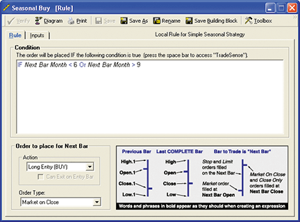
FIGURE 9: Trade NAVIGATOR, SOYBEAN TRADING SYSTEM. Here is how to set up the buy rule for the seasonal trading system.
We have already provided the strategies discussed in this article as a special downloadable file for Trade Navigator. In Trade Navigator, click on the blue phone icon, select “Download Special File,” type in “SC1109,” and click on the Start button.
![]() NINJATRADER: SEASONAL CHANNEL BREAKOUT SYSTEM
NINJATRADER: SEASONAL CHANNEL BREAKOUT SYSTEM
The trading system discussed in Markos Katsanos’ article in this issue, “A Seasonal System For Trading Soybean Futures,” has been implemented as a sample strategy available for download at www.ninjatrader.com/SC/November2009SC.zip. Please also be sure to import the data files available at www.ninjatrader.com/SC/November2009Data.zip.
Once you have that downloaded, from within the NinjaTrader Control Center window, select the menu File > Utilities > Import NinjaScript and select the “November2009SC” file. This strategy is for NinjaTrader version 6.5 or greater. To import the data files, export them from the zip and then go to File > Historical Data > Import and select the data files.
You can review the strategy’s source code by selecting the menu Tools > Edit NinjaScript > Strategy from within the NinjaTrader Control Center window and selecting “SoybeanSeasonalChannelBreakout.”
NinjaScript indicators are compiled Dlls that run native, not interpreted, which provides you with the highest performance possible.
A sample chart implementing the strategy is shown in Figure 10.
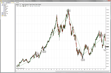
Figure 10: NINJATRADER, SEASONAL STRATEGY. The screenshot shows a partial view of several executed trades in the NinjaTrader Strategy Analyzer.
![]() UPDATA: SEASONAL CHANNEL BREAKOUT SYSTEM
UPDATA: SEASONAL CHANNEL BREAKOUT SYSTEM
This Traders’ Tip is based on the article by Markos Katsanos in this issue, “A Seasonal System For Trading Soybean Futures.”
In the article, Katsanos expands on a simple seasonal trading system by adding a channel breakout rule to obtain entry and exit signals within the appropriate seasonal time periods. He further adds a protective exit condition that closes long positions when the slope of the relative strength between current price and the average seasonal drops below a certain percentage.
The Updata code for Katsanos’ system is in the Updata System Test Library and may be downloaded by clicking the Custom menu and then “System Test Library.” Those who cannot access the library due to firewall issues may paste the code shown below into the Updata Custom editor and save it.
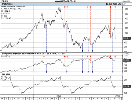
FIGURE 11: UPDATA, SOYBEAN TRADING SYSTEM. This chart shows the soybean continuous contract, with the equity line showing the entry and exit points, and the soybean seasonal data below. The solid arrows are long trade entry and exits and the hollow arrows are the short trades.
The system is run on the soybean continuous futures contract and uses the dollar index as well as soybean seasonal data, which may be obtained from the Stocks & Commodities website (www.traders.com) or by using Updata’s seasonal calculator. See Figure 11 for an example implementation of the system; system test results are shown in Figure 12.
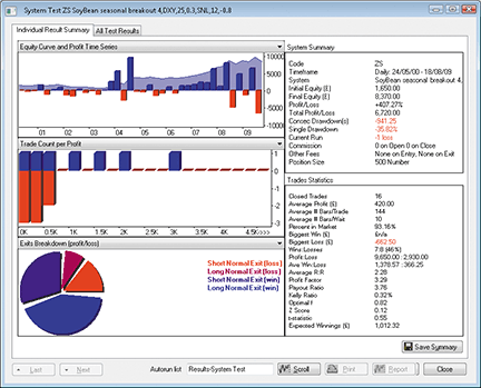
FIGURE 12: UPDATA, TEST RESULTS. Here are the system test results using Katsanos’s soybean data and seasonal data.
NAME SoyBean Seasonal Breakout System

  PARAMETER “Channel Length” #LENGTH=4
  PARAMETER “Dollar Index” ~CURRENCY=Select
  PARAMETER “Currency Slope Bars” #CURRENCYSLOPE=25
  PARAMETER “Currency Slope Filter” @CURRENCYFILTER=.3
  PARAMETER “Seasonal” ~SEASONAL=Select
  PARAMETER “Seasonal Slope Bars” #SEASONALSLOPE=12
  PARAMETER “Seasonal Slope Filter” @SEASONALFILTER=-0.8

  #SELLMONTH=6
  #BUYMONTH=9

  @SeasonalAdjusted=0
  @AveAdjusted=0
  @SeasonalRegression=0
  @CurrencyRegression=0

  #SeasonalBuy=0
  #SeasonalShort=0
  #Channel=4

  FOR #CURDATE=0 to #LASTDATE
  @SeasonalAdjusted=CLOSE/~SEASONAL
  @AveAdjusted=SGNL(@SeasonalAdjusted,3,E)

  IF #CURDATE>=#SEASONALSLOPE+3
  ‘ calculate the average slope on the LSR line of the seasonal average
  @SeasonalRegression=(LSR(@AveAdjusted,#SeasonalSlope,0,#SeasonalSlope)-LSR(@AveAdjusted,#SeasonalSlope,0,0))
  @SeasonalRegression=(@SeasonalRegression*100)/(#SeasonalSlope*LSR(@AveAdjusted,#SeasonalSlope,0,0))
  ENDIF

  IF #CURDATE>=#CURRENCYSLOPE
  ‘ calculate the average slope on the LSR line of the dollar index/currency average
  @CurrencyRegression=(LSR(~CURRENCY,#CurrencySlope,0,#CurrencySlope)-LSR(~CURRENCY,#CurrencySlope,0,0))
  @CurrencyRegression=(@CurrencyRegression*100)/(#CurrencySlope*LSR(~CURRENCY,#CurrencySlope,0,0))
  ENDIF

  IF ((#CURMONTH<#SELLMONTH) OR (#CURMONTH>#BUYMONTH)) AND (@SeasonalRegression>@SeasonalFilter) AND (@CurrencyRegression<@CurrencyFilter) AND (CLOSE>(PHIGH(CLOSE(1),#Channel)+2))
  BUY OPEN(-1)
  ENDIF
  IF ((#CURMONTH>#SELLMONTH) AND (#CURMONTH<=#BUYMONTH)) AND (@SeasonalRegression<-@SeasonalFilter) AND (@CurrencyRegression>-@CurrencyFilter) AND (CLOSE<(PLOW(CLOSE(1),#Channel)-2))
  SHORT OPEN(-1)
  ENDIF

  ‘ check for exits
  IF ORDERISOPEN>0
  IF (CLOSE<EAVE(15))
  IF @SeasonalRegression<@SeasonalFilter
  SELL OPEN(-1)
  ELSEIF SGNL(~CURRENCY,50,E)>HIST(SGNL(~CURRENCY,50,E),1) AND (@CurrencyRegression>@CurrencyFilter)
  SELL OPEN(-1)
  ENDIF
  ENDIF
  ELSEIF ORDERISOPEN<0
  IF (CLOSE>EAVE(15))
  IF @SeasonalRegression>-@SeasonalFilter
  COVER OPEN(-1)
  ELSEIF SGNL(~CURRENCY,50,E)<HIST(SGNL(~CURRENCY,50,E),1) AND (@CurrencyRegression<-@CurrencyFilter)
  COVER OPEN(-1)
  ENDIF
  ENDIF
  ENDIF

  NEXT
![]() UPDATA: THE PIVOT DETECTOR OSCILLATOR, SIMPLIFIED
UPDATA: THE PIVOT DETECTOR OSCILLATOR, SIMPLIFIED
This Traders’ Tip is based on the article by Giorgos Siligardos in the July 2009 issue of Stocks & Commodities, “The Pivot Detector Oscillator, Simplified.” The Pid oscillator is based on the relative strength index (Rsi) and Siligardos’ Pid signals. The observation is that the Rsi reaches different levels in a bull market compared to a bear market, so Pid signals are generated at different Rsi levels, depending on the market (Figure 13). To make Pid signals easier to spot, Siligardos created the Pid oscillator, where a buy signal is generated when the Pid oscillator crosses zero from below and a sell signal when it crosses 100 from above. Repeat buy and sell signals are possible.
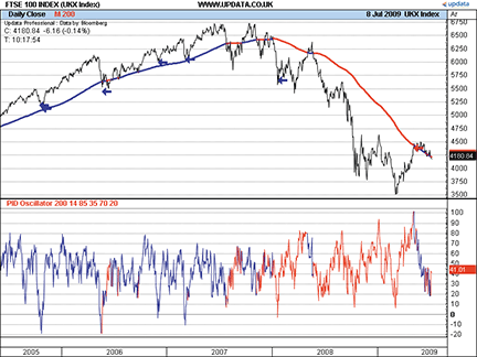
FIGURE 13: UPDATA, PID OSCILLATOR. This sample chart shows the FTSE 100 from Giorgos Siligardos’ July 2009 article with the PID oscillator using the standard periods and levels with blue and red arrows marking the buy and sell signals generated. The line color changes from blue to red to show the changes from bullish to bearish markets as defined by Siligardos.
To make the indicator more flexible, we have added parameters so the periods and key levels can be optimized. The code below is already in the Updata Custom Indicator Library and may be downloaded by clicking the Custom menu and then Custom Indicator Library. Those who cannot access the library due to firewall issues may copy the code below and paste it into the Updata Custom editor and save it.
  ‘ The PID Oscillator by Giorgos E. Siligardos
  ‘ September 2009 issue of S&C Magazine
  PARAMETER “Moving Average Period” #MA=200
  PARAMETER “RSI Period” #PERIOD=14
  PARAMETER “Bull Upper level” #BULLUP=85
  PARAMETER “Bull Lower level” #BULLDN=35
  PARAMETER “Bear Upper level” #BEARUP=70
  PARAMETER “Bear Lower level” #BEARDN=20
  DISPLAYSTYLE 2LINES

‘ PLOT = average superimposed (TOOL) on the main chart window
  INDICATORTYPE TOOL
  NAME “M” #MA

‘ PLOT2 = the oscillator itself which appears as its own chart window
  INDICATORTYPE2 CHART
  NAME2 PID Oscillator
  FOR #CURDATE=0 TO #LASTDATE
  @PLOT=MAVE(#MA)
  IF CLOSE>MAVE(#MA)
  @PLOT2=100*((RSI(#PERIOD)-#BULLDN)/(#BULLUP-#BULLDN))
  COLOR RGB(0,0,255)
  COLOR2 RGB(0,0,255)
  ELSE
  @PLOT2=100*((RSI(#PERIOD)-#BEARDN)/(#BEARUP-#BEARDN))
  COLOR RGB(255,0,0)
  COLOR2 RGB(255,0,0)
  ENDIF

  ‘ Buy when PID crosses up through zero
  IF @PLOT2>0 AND HIST(@PLOT2,1)<0
  DRAWIMAGE #CURDATE,CLOSE,Small Blue Arrow Left,RGB(0,0,255)
  ‘ Sell when PID crosses down through 100
  ELSEIF @PLOT2<100 AND HIST(@PLOT2,1)>100
  DRAWIMAGE #CURDATE,CLOSE,Small Red Arrow Left,RGB(255,0,0)
  ENDIF
  NEXT
![]() VT TRADER: FOUR-PERIOD LOOKBACK %R PAINTBAR SYSTEM
VT TRADER: FOUR-PERIOD LOOKBACK %R PAINTBAR SYSTEM
Our Traders’ Tip this month is inspired by Jim White’s article from the July 2009 issue of Stocks & Commodities, “Identifying Market Reversals.” In the article, White describes a method to help traders identify potential market reversals by combining four %R indicators, each with different lookback periods.
We’ll be offering this %R paintbar system for download in our client forums. The VT Trader instructions for recreating the aforementioned sample alert system are as follows:
- Navigator Window>Tools>Trading Systems Builder>[New] button
- In the Indicator Bookmark, type the following text for each field:
  Name: TASC - 11/2009 - 4-Period LookBack %R PaintBar System
  Short Name: tasc_4PRPBS
  Label Mask: TASC - 11/2009 - 4-Period LookBack %%R PaintBar System (%periods1%,%periods2%,%periods3%,%periods4%)
- In the Input Bookmark, create the following variables:
  [New] button... Name: periods1 , Display Name: %R Cycle 1 Periods , Type: integer , Default: 4
  [New] button... Name: periods2 , Display Name: %R Cycle 2 Periods , Type: integer , Default: 7
  [New] button... Name: periods3 , Display Name: %R Cycle 3 Periods , Type: integer , Default: 21
  [New] button... Name: periods4 , Display Name: %R Cycle 4 Periods , Type: integer , Default: 28
- In the Output Bookmark, create the following variables:
 [New] button...
  Var Name: PotentialBuyAlertPaintBar
  Name: Paint Bars for Potential Buy Alert
  * Checkmark: Highlights Enabled
  Select Highlights Tab
  Color: green
  [OK] button...
 [New] button...
  Var Name: PotentialSellAlertPaintBar
  Name: Paint Bars for Potential Sell Alert
  * Checkmark: Highlights Enabled
  Select Highlights Tab
  Color: pink
  [OK] button...
- In the Formula Bookmark, copy and paste the following formula:
//Provided By: Visual Trading Systems, LLC & Capital Market Services, LLC //Copyright (c): 2009 //Notes: July 2009 T.A.S.C. magazine //Notes: “Indentifying Market Reversals” by Him White} //Description: 4-period lookback %R PaintBar System //File: tasc_4PRPBS.vttrs {Williams %R Indicators} WR1:= vt_WilliamsR(periods1); WR2:= vt_WilliamsR(periods2); WR3:= vt_WilliamsR(periods3); WR4:= vt_WilliamsR(periods4); OB:= -20; OS:= -80; {Paint Bar Conditions} PotentialBuyAlertPaintBar:= ref(WR1,-1)<OS AND ref(WR1,-1)<WR1 AND WR2<OS AND WR3<OS AND WR4<OS; PotentialSellAlertPaintBar:= ref(WR1,-1)>OB AND ref(WR1,-1)>WR1 AND WR2>OB AND WR3>OB AND WR4>OB; - Click the “Save” icon to finish building the 4-Period Lookback %R paintbar system.
To attach the trading system to a chart (Figure 14), select the “Add Trading System” option from the chart’s contextual menu, select “TASC - 11/2009 - 4-Period LookBack %R PaintBar System” from the trading systems list, and click the [Add] button.

Figure 14: VT TRADER, %R PaintBar System. Here is the %R PaintBar system attached to a EUR/USD 10-minute candlestick chart.
To learn more about VT Trader, please visit www.cmsfx.com.
Risk disclaimer: Past performance is not indicative of future results. Forex trading involves a substantial risk of loss and may not be suitable for all investors.
![]() TRADE IDEAS: SEASONAL CHANNEL BREAKOUT SYSTEM
TRADE IDEAS: SEASONAL CHANNEL BREAKOUT SYSTEM
“When you discover you are riding a dead horse, the best strategy is to dismount.”—Comanche Indian wisdom
This Traders’ Tip is on the effect of seasonality in commodity futures, based on the article in this issue, “A Seasonal System For Trading Soybean Futures” by Markos Katsanos.
Seasonality can apply to different time frames, not just yearly time frames. To the extent that seasonality refers to predictable behaviors during certain periods, you could look at a single day as having seasonality — the open being harvest time!
Our model this month identifies a strong preference for a specific time of day (the open) and compares the same strategy if it were traded throughout the day. We discovered that the open provides for the best return. In fact, we liked the results as reported by our event-based backtesting tool, The OddsMaker, so much that we present the strategy, the backtests comparing two different time frames, and all the settings here.
  Description: “Strong Open Fade”
  Provided by:
  Trade Ideas (copyright © Trade Ideas LLC 2009). All rights reserved. For educational purposes only. Remember these are
  sketches meant to give an idea how to model a trading plan. Trade-Ideas.com and all individuals affiliated with this
  site assume no responsibilities for trading and investment results.
Type or copy/paste the following shortened string directly into a browser, then copy/paste the full-length link into Trade-Ideas Pro using the “Collaborate” feature (right-click in any strategy window):
https://bit.ly/DtOY3 (case sensitive)
FIGURE 15: TRADE IDEAS, ALERTS CONFIGURATION. This shows the combination of alerts and filters used to create the “Strong Open Fade” strategy in Trade Ideas.
This strategy also appears on the Trade Ideas blog at https://marketmovers.blogspot.com/, or you can build the strategy based on Figure 15, which shows the configuration of this strategy, where one alert and four filters are used with the following settings:
- Running-up now alert ($1)
- Min price = 10 ($)
- Max price = 50 ($)
- Max distance from inside market = 0.1 (%)
- Min daily volume = 50,000 (shares/day)
The definitions of these indicators appear here: https://www.trade-ideas.com/Help.html.
That’s the strategy, but what about the trading rules? How should the opportunities that the strategy finds be traded? We looked at two trading plans to backtest and compared the results.
To recap briefly, The OddsMaker doesn’t just look at a basket of stocks, à priori, to generate backtest results. Rather, it considers any stock that matches a desired pattern in the market, finds that stock, and applies the backtest’s ruleset before summing up the results into a detailed set of totals: win rate, average winner, average loser, net winnings, confidence factor.
FIGURE 16: TRADE IDEAS, OddsMaker backtesting configuration. Here is the OddsMaker backtesting configuration for the “Strong Open Fade” strategy.
In summary, this strategy trades only the first 10 minutes of the market after the open, selling short stocks that make at least a $1 jump upward in a matter of seconds. We evaluated several time frames, but were ultimately led to a hold time lasting only 10 minutes (it’s a coincidence that the holding time is the same as the trading window for taking any trades) with a stop value of $0.20 assigned and no predetermined profit target.
Here is what The OddsMaker tested for the past 15 days ended 9/11/2009 given the following trade rules:
- On each alert, sell short the symbol (price moves down to be a successful trade)
- Schedule an exit for the stocks 10 minutes after entry
- Trade only the first 10 minutes of the market session
- Exit the trade (cover) if the price moves up $0.20.
The OddsMaker summary provides the evidence of how well this strategy and our trading rules did. The settings are shown in Figure 16.
The results (last backtested for the 15-day period ended 09/11/2009) are as follows: This strategy generated 290 trades, of which 177 were profitable for a win rate of 61%. The average winning trade generated $0.41 in profit and the average loser lost $0.17. That’s more than a 2:1 win-to-loss ratio. The net winnings of using this strategy for 15 trading days generated $55.69 points. If you normally trade in 100-share lots, this strategy would have generated $5,569. The z-score or confidence factor that the next set of results will fall within this strategy’s average winner and loser is 100%.
We compared this backtested trading plan to others, holding everything the same except for the trading time in the market. We compared the strategy as if only the 12:00 noon ET–1:00 pm ET lunch hour were traded. The result was only three trades in 15 days for a small loss of $0.05. Trading the last 10 minutes generated no trades at all.
FIGURE 17: TRADE IDEAS, BACKTEST RESULTS. Here are the OddsMaker results for the “strong open fade” strategy.
Interestingly, trading the “strong open fade” strategy for the entire market session with our original backtested trading plan did yield very good, only slightly less-profitable results. Maybe a good pattern can withstand any season!
You can understand these backtest results (see Figure 17) from The OddsMaker in more detail by going to the online user manual at https://www.trade-ideas.com/OddsMaker/Help.html.
![]() MULTICHARTS: SOYBEAN SEASONAL CHANNEL BREAKOUT SYSTEM (KATSANOS ARTICLE CODE)
MULTICHARTS: SOYBEAN SEASONAL CHANNEL BREAKOUT SYSTEM (KATSANOS ARTICLE CODE)
Copyright 2009 by Markos Katsanos
The tests were carried out using MultiCharts 5.05 from TS Support (https://www.tssupport.com/multicharts/)
To recreate the tests, open a new chart window and insert the following symbols in the same order:
Soybeans E-CBOT continuous, Dollar Index (Data2), and the seasonal Data (Data3).
Seasonal data can be downloaded from the Stocks & Commodities website at www.traders.com. Then open the format symbol window, select the settings tab, and in the data range section, enter the starting and end dates from 6/7/2000 to 8/20/2009. (The starting date should be 50 days earlier than the actual test date in order to take into account the extra days needed to calculate all indicators before the system can start to produce signals.)
Then insert the channel breakout signal, open the Strategy Properties window, and fill in the commissions of $50 per trade (to take into account both commissions and slippage) and in the “Maximum bars back” box, enter 50 days.
{**************************************
  Strategy: SOYBEAN SEASONAL-CHANNEL BREAKOUT STRATEGY
  Provided By	: MARKOS KATSANOS Copyright 2009
  **************************************}
{LENGTH=Channel length in days,
  D1DXY=Days for the Dollar Index linear regression slope calculation
  D2SNL=Days for the Seasonal data linear regression slope calculation
  LRSNLSELL= Seasonal data linear regression slope per day
  LRSDXYSELL=Dollar index linear regression slope per day
  MASNL=Days for the seasonal exponential moving average sell/buytocover conditions
  MASELL=Days for the Soybean exponential moving average sell/buytocover conditions
  MADXY=Days for the Dollar Index moving average sell/buytocover conditions}
INPUTS:LENGTH(4),D1DXY(25),D2SNL(12),SELLMONTH(6),BUYMONTH(9),LRSNLSELL(-.8),LRSDXYSELL(.3),MASNL(15),MASELL(15),MADXY(50);
  VARIABLES:RS(0),LRSNL(0),S2(0),STOPL(0),SEASONALBUY(FALSE),
  SEASONALSHORT(FALSE),LRSDXY(0);
  IF BARNUMBER>3 THEN BEGIN
  RS=XAverage((C/CLOSE OF DATA3),3);
  END;
  IF BARNUMBER>D2SNL+3 THEN BEGIN
  LRSNL=(LINEARREGVALUE(RS,D2SNL,0)-LINEARREGVALUE(RS,D2SNL,D2SNL))/LINEARREGVALUE(RS,D2SNL,D2SNL)
  /D2SNL*100; END;
  IF BARNUMBER>D1DXY THEN BEGIN
  LRSDXY=(LINEARREGVALUE(CLOSE OF DATA2,D1DXY,0)-LINEARREGVALUE(CLOSE OF DATA2,D1DXY,D1DXY))
  /LINEARREGVALUE(CLOSE OF DATA2,D1DXY,D1DXY)/D1DXY*100;
  END;
  SEASONALBUY=Month(D)<SELLMONTH OR Month(D)>BUYMONTH;
  SEASONALSHORT=MONTH(D)>SELLMONTH AND MONTH(D)<BUYMONTH+1;
  {Buy&Short conditions}
  IF SEASONALBUY AND LRSDXY<LRSDXYSELL AND C>(HIGHEST(C[1],LENGTH)+2) AND LRSNL>LRSNLSELL THEN
  BUY (“BUY”)NEXT BAR AT OPEN;
  IF SEASONALSHORT AND C<LOWEST(C,LENGTH)[1]-2
  AND LRSDXY>-LRSDXYSELL AND LRSNL<-LRSNLSELL
  THEN sellshort (“SHORT”) NEXT BAR AT MARKET;
{Exit conditions}
  IF marketposition=1 AND barssinceentry>1 THEN begin
  IF C<XAverage(C,MASELL) AND LRSNL<LRSNLSELL
  THEN SELL(“LEXIT RS”) NEXT BAR AT OPEN; {RS with SNL Exit}
  IF C<XAverage(C,MASELL) AND XAverage(CLOSE OF DATA2,MADXY)>XAverage(CLOSE OF DATA2,MADXY)[1]
  AND LRSDXY>LRSDXYSELL THEN SELL(“LEXIT DXY”) NEXT BAR AT OPEN;
  {DXY Exit}
  END;
IF marketposition=-1 AND barssinceentry>1 THEN begin
  IF C>XAverage(C,MASELL) AND LRSNL>-LRSNLSELL
  THEN buytocover (“SEXIT RS”) NEXT BAR AT MARKET;
  IF C>XAverage(C,MASELL) AND XAverage(CLOSE OF DATA2,MADXY)<XAverage(CLOSE OF DATA2,MADXY)[1]
  AND CLOSE OF DATA3>XAverage(CLOSE OF DATA3,MASNL)THEN buytocover (“SEXIT DXY”)NEXT BAR AT MARKET;
  END;

Simple seasonal strategy
{**************************************
  Strategy	: SOYBEAN SIMLE DATE SEASONAL STRATEGY
  Provided By	: MARKOS KATSANOS Copyright 2009
  **************************************}
  Inputs: SELLMONTH(6),BUYMONTH(9);
  VARIABLES:SEASONALBUY(FALSE),SEASONALSHORT(FALSE);
  SEASONALBUY=Month(D)<SELLMONTH OR Month(D)>BUYMONTH;
  SEASONALSHORT=MONTH(D)>SELLMONTH AND MONTH(D)<BUYMONTH+1;
If  SEASONALBUY THEN Buy (“buy”) THIS BAR ON CLOSE ;
  If  SEASONALSHORT THEN SELLSHORT (“SHORT”) THIS BAR ON CLOSE;

Simple moving average crossover strategy
inputs: FastLength( 18 ), SlowLength( 120 ) ;
  variables: MAS( 0 ), MAL( 0 ) ;
MAS = AverageFC( C, FastLength ) ;
  MAL = AverageFC( C, SlowLength ) ;
IF CURRENTBAR>SLOWLENGTH THEN BEGIN
  if MAS CROSSES OVER MAL then
  Buy ( “MACrossLE” ) next bar at market ;
  if MAS CROSSES UNDER MAL then
  Sell Short ( “MACrossSE” ) next bar at market ;
  END;
Note: Test results may vary according to your data provider and the method used to create continuous contracts. For these tests, I used the following data from Reuters: Soybean E-CBOT Continuous Contract (Reuters Symbol:@:ZSc1) and the Dollar Index (.DXY).