TRADING TECHNIQUES
About Parameter-Sensitive Indicators
Signal Processing Basics
Part 2
This is the second of a series of articles that examine stock price analysis using the mathematical methods of signal processing. Here you will learn about tools for detecting trends and smoothing them.
In the first part of this series, I proposed a model for price time series that could be analyzed using signal processing techniques:
Equation 1-1a:
P = Constant + trend + cyclical components + noise
or
Equation 1-1b:
P = c + f(t)trend + Sum[f(t)cycles ] + f(t)noise
One way to view this model of price action is to think in terms of the frequency of price changes. From a frequency perspective, this model can be restated in terms of:
- Low-frequency components c + f(t)trend + f(t)cycles where cycles terms have very long periods compared to the trading horizon
- f(t)cycles terms where the cycle period is on the same order of magnitude of the trading horizon
- f(t)cycles + noise where the high-frequency and noise terms result in price variations that are much shorter than our trading horizon.
In the first article of the series, I described the cyclical components along with analysis tools such as the fast Fourier transform (Fft). In this second article, I will discuss the trend and low-frequency components and introduce tools for trend detection and low-pass filtering (smoothing).
The emphasis on the trend and low-frequency components is tied closely to trading strategies based on the Dow theory that describes the market in terms of trends of different length:
- Long-term major trend: Bullish — prices rising, or bearish — prices falling for prolonged period and change in value of more than 20%
- Intermediate secondary trend: A correction or reaction to the primary trend
- Short-term minor trend: A temporary decrease during bull markets or a temporary rise during a bear market.
What do we want to accomplish with this information?

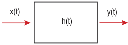
Figure 1: schematic of a signal filter. A signal filter takes an input data signal x(t) and provides a frequency and amplitude altered signal y(t) as its output based on the filter impulse response characteristic h(t).