OPTIONS
Part 2 Of Two Parts
Choosing Optimal Moneyness
In his previous article, Giorgos Siligardos demonstrated how the movement of the underlying, the implied volatility changes, and the passage of time all affect the price of options. This time, he shows how a simple computerized approach to the problem of choosing the optimal moneyness could be what you’re looking for.
In “Buying The Optimal Moneyness,” I showed how the movement of the underlying, the implied volatility changes, and the passage of time affect the price of out-of-the-money, at-the-money, and in-the-money options. In this article, I will show you a simple computerized approach to the problem of choosing the optimal moneyness to buy. For the rest of the article I will deal with European options on broad stock market indexes.
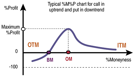
To identify what kind of options are the best to hold when a market trend is expected, we can use the Black-Scholes model and calculate the expected percentage profit in various cases. The results can then be plotted in charts that I call “theoretical %moneyness–%profit” charts (or simply, “%M%P charts”) and produce a curve (namely, the “%M%P curve”). The y-axis of a %M%P chart shows percentage profits, while the x-axis shows the “%moneyness” of an option (that is, how much percentage in-the-money the option is) as a percentage of its spot price.
- Example 1: A %moneyness of 5% means that the option is 5% in-the-money (ITM), so if the option is a call and the spot price is, say, 1000, then its strike is 950. If the option is a put, then its strike is 1050.
- Example 2: A %moneyness of -5% means that the option is -5% ITM, so it is 5% out-of-the-money (OTM). If the option is a call and the spot price is 1000, then its strike is 1050, whereas if the option is a put, then its strike is 950.
- Example 3: A zero %moneyness means that the option is at-the-money (ATM).
It is clear that an option has positive %moneyness if it is ITM, zero %moneyness if it is ATM, and negative %moneyness if it is OTM. To calculate the values of a %M%P curve:
- You assume an option, a market trend, and market data for the Black-Scholes model for both the start and the end of this trend.
- You use the Black-Scholes model (see the sidebar “Black-Scholes Fair Value Formulas”) to find the fair prices P1 and P2 of the option at the start and at the end of the trend, respectively, and you calculate the percentage profit/loss: 100%*(P2-P1)/P1.
- You repeat the calculations for various strike prices of the option (that is, for various %moneynesses), keeping the time to maturity constant.

FIGURE 1: TYPICAL %M%P CHARTS FOR CALLS IN UPTREND AND PUTS IN DOWNTREND. This is the typical %M%P curve for calls in a market uptrend, where the IV normally falls and for puts in a market downtrend, where the IV advances. There are two critical %moneynesses in the chart. The first is the optimal %moneyness (OM), which gives the highest percentage profit, and the second is the least %moneyness, which doesn’t produce losses (breakeven %moneyness, or simply BM).