TRADERS’ TIPS
June 2019

For this month’s Traders’ Tips, the focus is John Ehlers’ article in this issue, “Fourier Series Model Of The Market.” Here, we present the June 2019 Traders’ Tips code with possible implementations in various software.
You can right-click on any chart to open it in a new tab or window and view it at it’s originally supplied size, often much larger than the version printed in the magazine.
The Traders’ Tips section is provided to help the reader implement a selected technique from an article in this issue or another recent issue. The entries here are contributed by software developers or programmers for software that is capable of customization.

TRADESTATION: JUNE 2019
In “Fourier Series Model Of The Market” in this issue, author John Ehlers introduces a Fourier series indicator designed to help traders identify cycles in the market. According to the author, the approach based on five principles outlined by J.M. Hurst in his 1970 book allows the determinization of a security’s primary cycle period and gives a faithful picture of market activity.
Here, we are providing TradeStation EasyLanguage code for an indicator and strategy based on Ehlers’ concepts described in the article. This code can be downloaded by visiting our TradeStation and EasyLanguage support forum at the link provided after the following code listing.
Indicator: Fourier Series Indicator
// TASC JUN 2019
// Fourier Series Analysis
// (C) 2005-2018 John F. Ehlers

inputs:
	Fundamental( 20 ) ;

variables:
	Bandwidth(.1),
	G1( 0 ), S1( 0 ), L1( 0 ), BP1( 0 ), Q1( 0 ), P1( 0 ),
	G2( 0 ), S2( 0 ), L2( 0 ), BP2( 0 ), Q2( 0 ), P2( 0 ),
	G3( 0 ), S3( 0 ), L3( 0 ), BP3( 0 ), Q3( 0 ), P3( 0 ),
	count( 0 ),	Wave( 0 ), ROC( 0 ) ;

//compute filter coefficients once
once
begin
	L1 = Cosine( 360 / Fundamental ) ;
	G1 = Cosine( Bandwidth * 360 / Fundamental ) ;
	S1 = 1 / G1 - SquareRoot( 1 / ( G1 * G1 ) - 1 ) ;
	L2 = Cosine( 360 / ( Fundamental / 2 ) ) ;
	G2 = Cosine( Bandwidth * 360 / ( Fundamental / 2 ) ) ;
	S2 = 1 / G2 - SquareRoot( 1 / ( G2 * G2 ) - 1 ) ;
	L3 = Cosine( 360 / ( Fundamental / 3 ) ) ;
	G3 = Cosine( Bandwidth * 360 / ( Fundamental / 3 ) ) ;
	S3 = 1 / G3 - SquareRoot( 1 / ( G3 * G3 ) - 1 ) ;
end ;

//Fundamental Band-Pass
BP1 = .5 * ( 1 - S1) * ( Close - Close[2] )
	+ L1 * ( 1 + S1 ) * BP1[1] - S1 * BP1[2] ;
if CurrentBar  <= 3 then
	BP1 = 0 ;

//Fundamental Quadrature
Q1 = ( Fundamental / 6.28 ) * ( BP1 - BP1[1] ) ;
if CurrentBar <= 4 then
	Q1 = 0 ;

//Second Harmonic Band-Pass
BP2 = .5 * ( 1 - S2 ) * ( Close - Close[2] )
	+ L2 * ( 1 + S2 ) * BP2[1] - S2 * BP2[2] ;
if CurrentBar <= 3 then
	BP2 = 0 ;

//Second Harmonic Quadrature
Q2 = ( Fundamental / 6.28 ) * ( BP2 - BP2[1] ) ;
if CurrentBar <= 4 then
	Q2 = 0 ;

//Third Harmonic Band-Pass
BP3 = .5 * ( 1 - S3 ) * ( Close - Close[2] )
	+ L3 * ( 1 + S3 ) * BP3[1] - S3 * BP3[2] ;
if CurrentBar <= 3 then
	BP3 = 0 ;

//Third Harmonic Quadrature
Q3 = ( Fundamental / 6.28 ) * ( BP3 - BP3[1] ) ;
if CurrentBar <= 4 then
Q3 = 0 ;

//Sum power of each harmonic at
//each bar over the Fundamental period
P1 = 0 ;
P2 = 0 ;
P3 = 0 ;
For count = 0 to Fundamental - 1
begin
	P1 = P1 + BP1[count] * BP1[count]
		+ Q1[count] * Q1[count] ;
	P2 = P2 + BP2[count] * BP2[count]
		+ Q2[count] * Q2[count] ;
	P3 = P3 + BP3[count] * BP3[count]
		+ Q3[count] * Q3[count] ;
end ;

//Add the three harmonics together
//using their relative amplitudes
If P1 <> 0 then
	Wave = BP1 + SquareRoot( P2 / P1 ) * BP2
		+ SquareRoot( P3 / P1 ) * BP3 ;

Plot1( Wave );
Plot2( 0 );

//Optional cyclic trading signal
//Rate of change crosses zero at
//cyclic turning points
ROC = ( Fundamental / 12.57 ) *
	( Wave - Wave[2] ) ;
Plot3( ROC ) ;


Strategy: Fourier Series Strategy
// TASC JUN 2019
// Fourier Series Analysis
// (C) 2005-2018 John F. Ehlers

inputs:
	Fundamental( 20 ) ;

variables:
	Bandwidth(.1),
	G1( 0 ), S1( 0 ), L1( 0 ), BP1( 0 ), Q1( 0 ), P1( 0 ),
	G2( 0 ), S2( 0 ), L2( 0 ), BP2( 0 ), Q2( 0 ), P2( 0 ),
	G3( 0 ), S3( 0 ), L3( 0 ), BP3( 0 ), Q3( 0 ), P3( 0 ),
	count( 0 ),	Wave( 0 ), ROC( 0 ) ;

//compute filter coefficients once
once
begin
	L1 = Cosine( 360 / Fundamental ) ;
	G1 = Cosine( Bandwidth * 360 / Fundamental ) ;
	S1 = 1 / G1 - SquareRoot( 1 / ( G1 * G1 ) - 1 ) ;
	L2 = Cosine( 360 / ( Fundamental / 2 ) ) ;
	G2 = Cosine( Bandwidth * 360 / ( Fundamental / 2 ) ) ;
	S2 = 1 / G2 - SquareRoot( 1 / ( G2 * G2 ) - 1 ) ;
	L3 = Cosine( 360 / ( Fundamental / 3 ) ) ;
	G3 = Cosine( Bandwidth * 360 / ( Fundamental / 3 ) ) ;
	S3 = 1 / G3 - SquareRoot( 1 / ( G3 * G3 ) - 1 ) ;
end ;

//Fundamental Band-Pass
BP1 = .5 * ( 1 - S1) * ( Close - Close[2] )
	+ L1 * ( 1 + S1 ) * BP1[1] - S1 * BP1[2] ;
if CurrentBar  <= 3 then
	BP1 = 0 ;

//Fundamental Quadrature
Q1 = ( Fundamental / 6.28 ) * ( BP1 - BP1[1] ) ;
if CurrentBar <= 4 then
	Q1 = 0 ;

//Second Harmonic Band-Pass
BP2 = .5 * ( 1 - S2 ) * ( Close - Close[2] )
	+ L2 * ( 1 + S2 ) * BP2[1] - S2 * BP2[2] ;
if CurrentBar <= 3 then
	BP2 = 0 ;

//Second Harmonic Quadrature
Q2 = ( Fundamental / 6.28 ) * ( BP2 - BP2[1] ) ;
if CurrentBar <= 4 then
	Q2 = 0 ;

//Third Harmonic Band-Pass
BP3 = .5 * ( 1 - S3 ) * ( Close - Close[2] )
	+ L3 * ( 1 + S3 ) * BP3[1] - S3 * BP3[2] ;
if CurrentBar <= 3 then
	BP3 = 0 ;

//Third Harmonic Quadrature
Q3 = ( Fundamental / 6.28 ) * ( BP3 - BP3[1] ) ;
if CurrentBar <= 4 then
Q3 = 0 ;

//Sum power of each harmonic at
//each bar over the Fundamental period
P1 = 0 ;
P2 = 0 ;
P3 = 0 ;
For count = 0 to Fundamental - 1
begin
	P1 = P1 + BP1[count] * BP1[count]
		+ Q1[count] * Q1[count] ;
	P2 = P2 + BP2[count] * BP2[count]
		+ Q2[count] * Q2[count] ;
	P3 = P3 + BP3[count] * BP3[count]
		+ Q3[count] * Q3[count] ;
end ;

//Add the three harmonics together
//using their relative amplitudes
If P1 <> 0 then
	Wave = BP1 + SquareRoot( P2 / P1 ) * BP2
		+ SquareRoot( P3 / P1 ) * BP3 ;

//Rate of change crosses zero at
//cyclic turning points
ROC = ( Fundamental / 12.57 ) *
	( Wave - Wave[2] ) ;

if ROC crosses over 0 then
	Buy next bar at Market
else if ROC crosses under 0 then
	SellShort next bar at Market ;
To download the EasyLanguage code, please visit our TradeStation and EasyLanguage support forum. The files for this article can be found here: https://community.tradestation.com/Discussions/Topic.aspx?Topic_ID=156727. The filename is “TASC_JUN2019.ZIP.” For more information about EasyLanguage in general, please see https://www.tradestation.com/EL-FAQ.
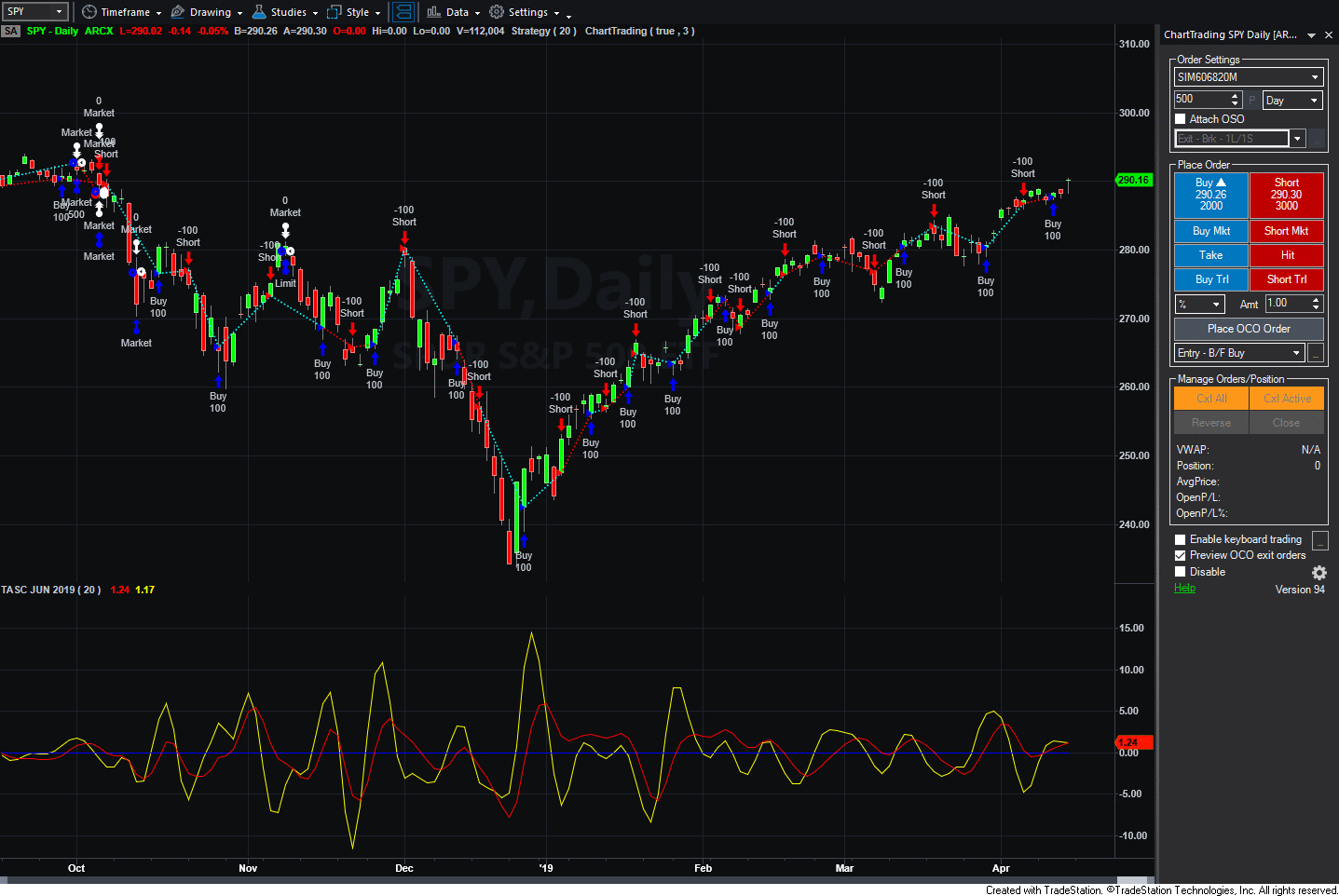
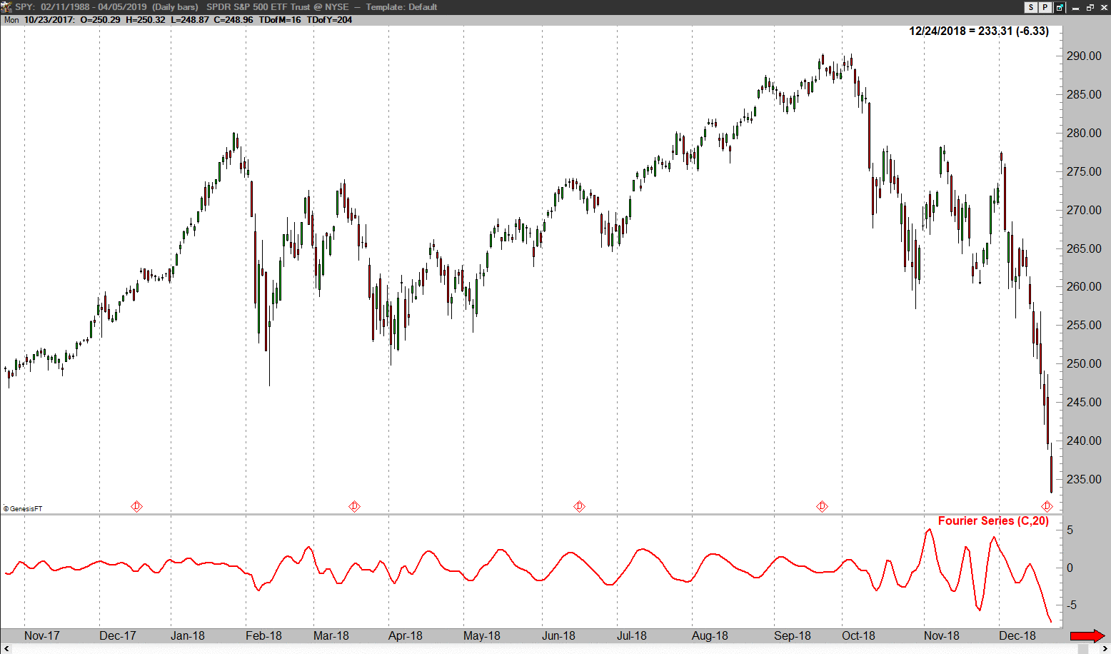
A sample chart is shown in Figure 1.

FIGURE 1: TRADESTATION. This shows a daily chart of SPY with the Fourier series indicator and strategy applied.
This article is for informational purposes. No type of trading or investment recommendation, advice, or strategy is being made, given, or in any manner provided by TradeStation Securities or its affiliates.
—Doug McCrary
TradeStation Securities, Inc.
www.TradeStation.com
BACK TO LIST

METASTOCK: JUNE 2019
John Ehlers’ article in this issue, “Fourier Series Model Of The Market,” explains how to reduce market action to a sinewave using Fourier series analysis. The MetaStock formula for that indicator is given here.
Fourier Series Analysis

x:= Input("fundemental cycle length", 2, 100, 20);
bw:= 0.1; {bandwidth}
L1:= Cos(360/x);
G1:= Cos((bw*360)/x);
S1:= 1/G1 - Sqrt(1/(G1*G1) -1);
L2:= Cos( 360 / (x/2));
G2:= Cos((bw*360)/(x/2));
S2:= 1/G2 - Sqrt(1/(G2*G2) -1);
L3:= Cos( 360 / (x/3));
G3:= Cos((bw*360)/(x/3));
S3:= 1/G3 - Sqrt(1/(G3*G3) -1);
{fundemental band pass}
BP1:= .5*(1-S1)*(C-Ref(C,-2)) + L1*(1+S1)*PREV - S1*Ref(PREV,-1);
Q1:= (x/6.28)*(BP1-Ref(BP1,-1));
{second harmonic band pass}
BP2:= .5*(1-S2)*(C-Ref(C,-2)) + L2*(1+S2)*PREV - S2*Ref(PREV,-1);
Q2:= (x/6.28)*(BP2-Ref(BP2,-1));
{third harmonic band pass}
BP3:= .5*(1-S3)*(C-Ref(C,-2)) + L3*(1+S3)*PREV - S3*Ref(PREV,-1);
Q3:= (x/6.28)*(BP3-Ref(BP3,-1));
{final calculations}
p1:= Sum((BP1*BP1) + (Q1*Q1), x);
p2:= Sum((BP2*BP2) + (Q2*Q2), x);
p3:= Sum((BP3*BP3) + (Q3*Q3), x);
BP1 + Sqrt(p2/p1)*BP2 + Sqrt(p3/p1)*BP3;
—William Golson
MetaStock Technical Support
www.metastock.com
BACK TO LIST

THINKORSWIM: JUNE 2019
We have put together a study based on the article “Fourier Series Model Of The Market” in this issue by John Ehlers. We built the referenced study and strategy by using our proprietary scripting language, thinkScript. To ease the loading process, simply click on https://tos.mx/vDTSrd and then choose view thinkScript study and name it “fourierseriesindicator.” This can then be added to your chart from the edit study and strategies menu within thinkorswim.
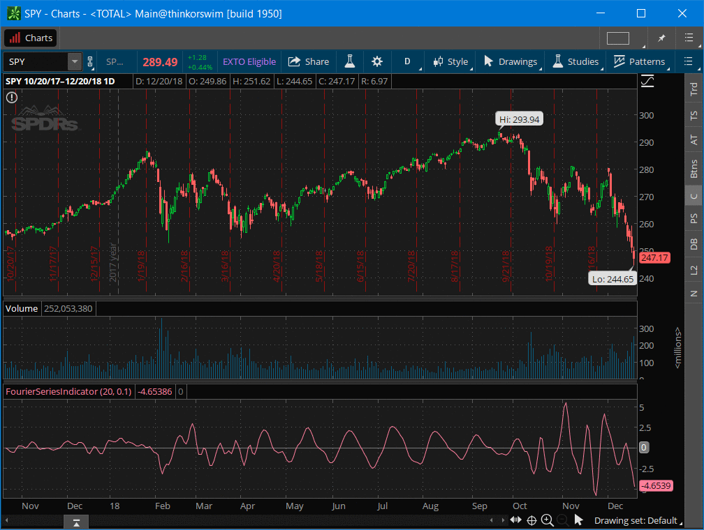
The study can be seen in Figure 2, set to display one-day candles for the date range of October 20, 2017 through December 20, 2018. See John Ehlers’ article in this issue for more details on how to interpret the study.

FIGURE 2: THINKORSWIM. This sample thinkorswim chart displays the study on one-day candles for the date range 10/20/2017–12/20/2018.
—thinkorswim
A division of TD Ameritrade, Inc.
www.thinkorswim.com
BACK TO LIST

eSIGNAL: JUNE 2019
For this month’s Traders’ Tip, we’ve provided the study Fourier_Series_Indicator.efs based on the article in this issue by John Ehlers, “Fourier Series Model Of The Market.” This study can be used to describe the cycles present in a market.
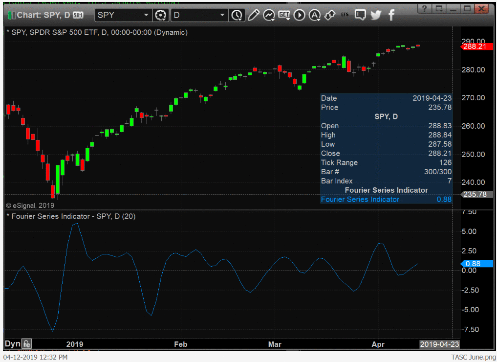
The study contains formula parameters that may be configured through the edit chart window (right-click on the chart and select “edit chart”). A sample chart is shown in Figure 3.

FIGURE 3: eSIGNAL. Here is an example of the study plotted on a daily chart of SPY.
To discuss this study or download a complete copy of the formula code, please visit the EFS library discussion board forum under the forums link from the support menu at www.esignal.com or visit our EFS KnowledgeBase at https://www.esignal.com/support/kb/efs/. The eSignal formula script (EFS) is also available for copying & pasting below.
/*********************************
Provided By:
Copyright 2019 Intercontinental Exchange, Inc. All Rights Reserved.
eSignal is a service mark and/or a registered service mark of Intercontinental Exchange, Inc.
in the United States and/or other countries. This sample eSignal Formula Script (EFS)
is for educational purposes only.
Intercontinental Exchange, Inc. reserves the right to modify and overwrite this EFS file with each new release.

Description:
   Fourier series Model Of The Market
   by John F. Ehlers


Version:            1.00  04/08/2019

Formula Parameters:                     Default:
Fundamental                             20


Notes:
The related article is copyrighted material. If you are not a subscriber
of Stocks & Commodities, please visit www.traders.com.

**********************************/


var fpArray = new Array();

function preMain(){
    setPriceStudy(false);
    setStudyTitle("Fourier Series Indicator");
    setCursorLabelName("Fourier Series Indicator");
    setPlotType(PLOTTYPE_LINE);

    var x = 0;
    fpArray[x] = new FunctionParameter("Fundamental", FunctionParameter.NUMBER);
	with(fpArray[x++]){
        setName("Fundamental");
        setLowerLimit(1);
        setDefault(20);
    }

}

var bInit = false;
var bVersion = null;
var xClose = null;
var Bandwidth = 0.1;
var G1 = 0;
var S1 = 0;
var L1 = 0;
var BP1 = 0;
var Q1 = 0;
var P1 = 0;
var G2 = 0;
var S2 = 0;
var L2 = 0;
var BP2 = 0;
var Q2 = 0;
var P2 = 0;
var G3 = 0;
var S3 = 0;
var L3 = 0;
var BP3 = 0;
var Q3 = 0;
var P3 = 0;
var Wave = 0;
var vBP1 = [];
var vBP2 = [];
var vBP3 = [];
var vQ1 = [];
var vQ2 = [];
var vQ3 = [];
var fNewBar = null;


function main(Fundamental){
    if (bVersion == null) bVersion = verify();
    if (bVersion == false) return;

    if (getBarState() == BARSTATE_ALLBARS){
        bInit = false;
    }

    if (getCurrentBarCount() < Fundamental) {

        vBP1.unshift(0);
        vBP2.unshift(0);
        vBP3.unshift(0)
        vQ1.unshift(0)
        vQ2.unshift(0)
        vQ3.unshift(0)
        return;

    }

    if (!bInit){

        xClose = close();
        L1 = Math.cos(2 * Math.PI / Fundamental);
        L2 = Math.cos(2 * Math.PI / (Fundamental / 2));
        L3 = Math.cos(2 * Math.PI / (Fundamental / 3));
        G1 = Math.cos(Bandwidth * 2 * Math.PI / Fundamental);
        G2 = Math.cos(Bandwidth * 2 * Math.PI / (Fundamental / 2));
        G3 = Math.cos(Bandwidth * 2 * Math.PI / (Fundamental / 3));
        S1 = 1 / G1 - Math.sqrt(1 / (G1*G1) - 1);
        S2 = 1 / G2 - Math.sqrt(1 / (G2*G2) - 1);
        S3 = 1 / G3 - Math.sqrt(1 / (G3*G3) - 1);

        addBand(0, PS_DASH, 1, Color.grey, 0);
        bInit = true;
    }

    fNewBar = false;
    P1 = 0;
    P2 = 0;
    P3 = 0;

    if (getBarState() == BARSTATE_NEWBAR) fNewBar = true;
    if (!fNewBar) {
        vBP1.shift();
        vBP2.shift();
        vBP3.shift();
        vQ1.shift();
        vQ2.shift();
        vQ3.shift();
    }

    if (getCurrentBarCount() <= 3) {
        vBP1.unshift(0);
        vBP2.unshift(0);
        vBP3.unshift(0);
    }
    else {
        vBP1.unshift(0.5 * (1 - S1)*(xClose.getValue(0) - xClose.getValue(-2)) + L1*(1 + S1)*vBP1[0] - S1*vBP1[1]);
        vBP2.unshift(0.5 * (1 - S2)*(xClose.getValue(0) - xClose.getValue(-2)) + L2*(1 + S2)*vBP2[0] - S2*vBP2[1]);
        vBP3.unshift(0.5 * (1 - S3)*(xClose.getValue(0) - xClose.getValue(-2)) + L3*(1 + S3)*vBP3[0] - S3*vBP3[1]);
    }

    if (getCurrentBarCount() <= 4) {
        vQ1.unshift(0);
        vQ2.unshift(0);
        vQ3.unshift(0);
    }
    else {
        vQ1.unshift((Fundamental / 6.28)*(vBP1[0] - vBP1[1]));
        vQ2.unshift((Fundamental / 6.28)*(vBP2[0] - vBP2[1]));
        vQ3.unshift((Fundamental / 6.28)*(vBP3[0] - vBP3[1]));
    }

    for (var i = 0; i < Fundamental; i++) {
        P1 = P1 + vBP1[i]*vBP1[i] + vQ1[i]*vQ1[i];
        P2 = P2 + vBP2[i]*vBP2[i] + vQ2[i]*vQ2[i];
        P3 = P3 + vBP3[i]*vBP3[i] + vQ3[i]*vQ3[i];
    }
    Wave = Calc_Ret(0, vBP1, vBP2, vBP3, P1, P2, P3);

    return Wave
}


function Calc_Ret(V, vBP1, vBP2, vBP3, P1, P2, P3){
    if (P1 == 0) return;
    var vWave = vBP1[0 + V] + Math.sqrt(P2 / P1)*vBP2[0 + V] + Math.sqrt(P3 / P1)*vBP3[0 + V];
    return vWave;
}


function verify(){
    var b = false;
    if (getBuildNumber() < 779){

        drawTextAbsolute(5, 35, "This study requires version 10.6 or later.",
            Color.white, Color.blue, Text.RELATIVETOBOTTOM|Text.RELATIVETOLEFT|Text.BOLD|Text.LEFT,
            null, 13, "error");
        drawTextAbsolute(5, 20, "Click HERE to upgrade.@URL=https://www.esignal.com/download/default.asp",
            Color.white, Color.blue, Text.RELATIVETOBOTTOM|Text.RELATIVETOLEFT|Text.BOLD|Text.LEFT,
            null, 13, "upgrade");
        return b;
    }
    else
        b = true;

    return b;
}
—Eric Lippert
eSignal, an Interactive Data company
800 779-6555, www.eSignal.com
BACK TO LIST

WEALTH-LAB: JUNE 2019
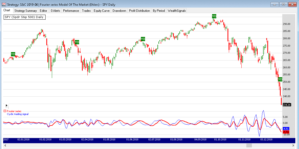
The FourierSeries indicator presented by John Ehlers in his article in this issue, “Fourier Series Model Of The Market,” represents market activity based on analysis principles established by J.M. Hurst. It does so by applying a set of band-pass filters.
In Wealth-Lab, install (or update) the TASCIndicators library to its most-recent version from our website or by using the built-in Extension Manager. Once you see the “Fourier series” and “Fourier cyclic trading signal” indicators listed under the TASC Magazine Indicators group, they’re ready for use in Wealth-Lab.
In Figure 4, you can see an example of the indicators applied.

FIGURE 4: WEALTH-LAB. Here are the two Fourier-based indicators applied to a daily chart of SPY (data provided by Yahoo).
—Gene (Eugene) Geren, Wealth-Lab team
MS123, LLC
www.wealth-lab.com
BACK TO LIST

QUANTACULA: JUNE 2019
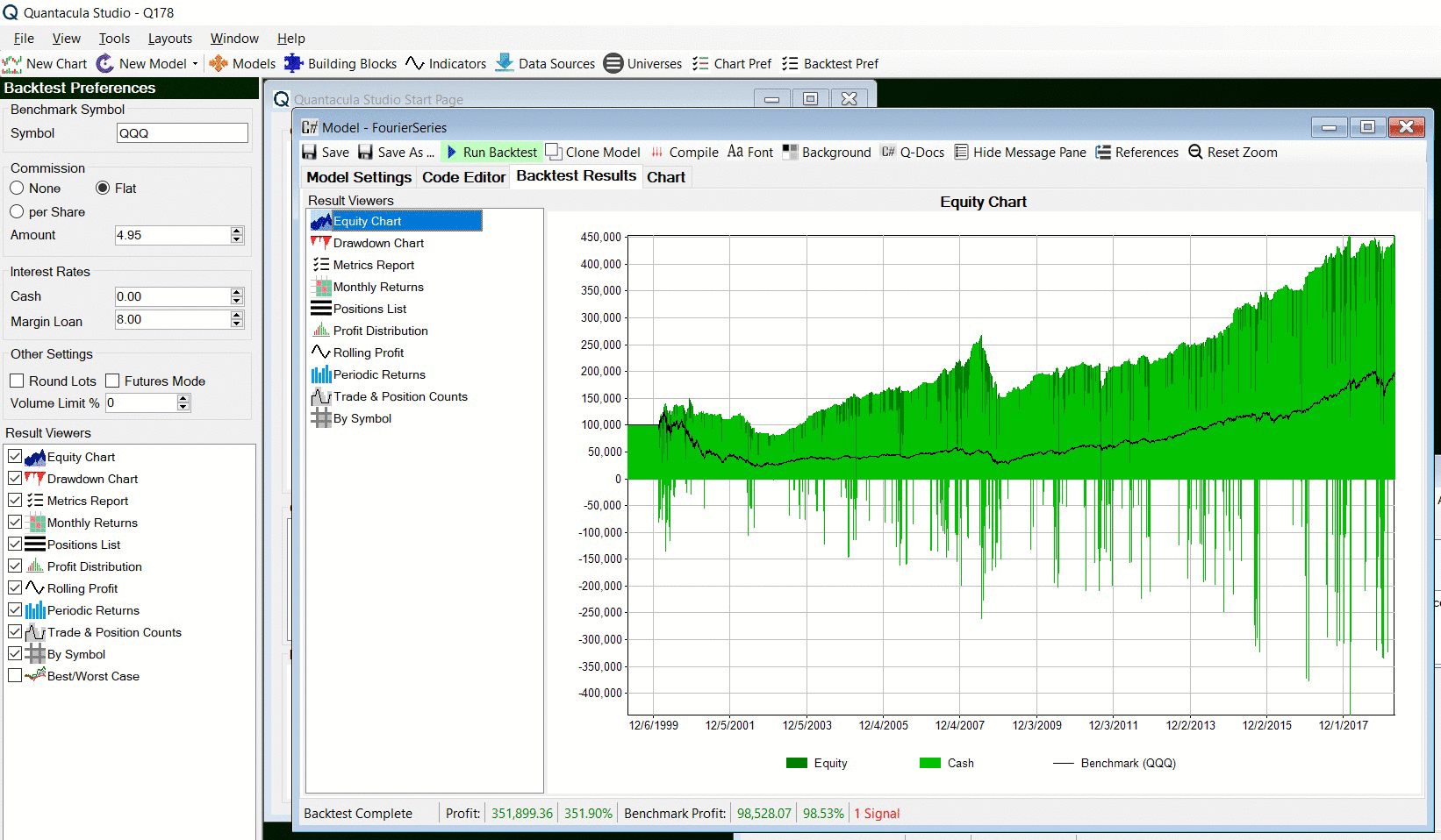
The FourierSeries indicator presented by John Ehlers in his article in this issue, “Fourier Series Model Of The Market,” is now available for Quantacula.com and Quantacula Studio from our TASC Extension library. We developed a simple system to exercise the indicator. Our trading model’s rules are:
- Buy next bar at market open when the FourierSeries(20) has reached a new 200-bar low and then turns up. This is an example of a “self-tuning” model, a concept we’ve been working with recently at Quantacula. Rather than establish an arbitrary oversold level, we use the historical data itself to look for an appropriate reversal level.
- Sell at a limit price equal to the highest two-bar high. We’ve found that this exit works well to capture small gains in markets that are due for an upside move, while reducing exposure.
We ran the model on the historical Nasdaq 100 stocks, corrected for survivorship bias by accounting for the stocks that came into and out of the index over time. We used $100,000 starting capital, a position size of 25% of equity, and a margin factor of 2 to 1. Over a 20-year backtest, the model returned 7.84% APR while the QQQ benchmark returned 3.49% APR. The model also had a win rate of nearly 70%.
Here is the Quantacula C# code for the self-tuning FourierSeries model:
using QuantaculaBacktest;
using QuantaculaCore;
using TASCExtensions;

namespace Quantacula
{
    public class MyModel : UserModelBase
    {
        //create indicators and other objects here, executed prior to main trading loop
        public override void Initialize(BarHistory bars)
        {
            fs = new FourierSeries(bars.Close, 20);
            PlotIndicator(fs);
            StartIndex = 201;
        }

        //execute strategy rules here, executed once for each bar in the backtest history
        public override void Execute(BarHistory bars, int idx)
        {
            if (LastPosition == null)
            {
                //is FS at its historical low, and turning up?
                double lowFS = fs.GetLowest(idx - 1, 200);
                if (fs[idx - 1] == lowFS)
                    if (fs.TurnsUp(idx))
                        PlaceTrade(bars, TransactionType.Buy, OrderType.Market);
            }
            else
            {
                //sell at 2 bar high
                PlaceTrade(bars, TransactionType.Sell, OrderType.Limit, bars.High.GetHighest(idx, 2));
            }
        }

        //declare private variables below
        private FourierSeries fs;
    }
}

FIGURE 5: QUANTACULA. This shows an example equity curve for the self-tuning FourierSeries model on Nasdaq 100 stocks.
—Dion Kurczek, Quantacula LLC
info@quantacula.com
www.quantacula.com
BACK TO LIST

NEUROSHELL TRADER: JUNE 2019
The Fourier market analysis indicator that John Ehlers describes in his article in this issue, “Fourier Series Model Of The Market,” can be easily implemented in NeuroShell Trader using NeuroShell Trader’s ability to call external dynamic linked libraries. Dynamic linked libraries (DLLs) can be written in C, C++, and Power Basic.
After moving the code given in Ehlers’ article to your preferred compiler and creating a DLL, you can insert the resulting indicator as follows:
- Select “New indicator …” from the insert menu.
- Choose the External Program & Library Calls
category.
- Select the appropriate External DLL Call indicator.
- Set up the parameters to match your DLL.
- Select the finished button.
Users of NeuroShell Trader can go to the Stocks & Commodities section of the NeuroShell Trader free technical support website to download a copy of this or any previous Traders’ Tips.
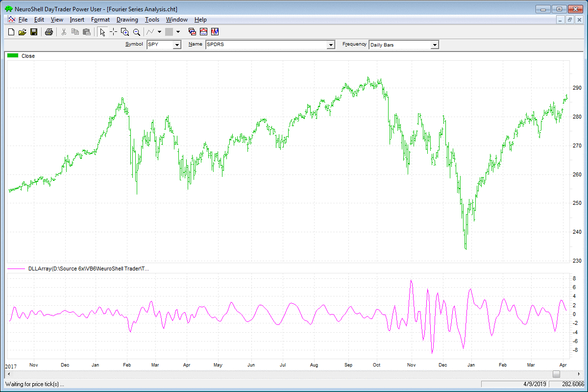
A sample chart is shown in Figure 6.

FIGURE 6: NEUROSHELL TRADER. This NeuroShell Trader chart shows the Fourier analysis on an SPY chart.
—Marge Sherald, Ward Systems Group, Inc.
301 662-7950, sales@wardsystems.com
www.neuroshell.com
BACK TO LIST

NINJATRADER: JUNE 2019
The Fourier series analysis indicator, as discussed in the article by John Ehlers in this issue, “Fourier Series Model Of The Market,” is available for download at the following links for NinjaTrader 8 and NinjaTrader 7:
Once the file is downloaded, you can import the indicator into NinjaTader 8 from within the control center by selecting Tools → Import → NinjaScript Add-On and then selecting the downloaded file for NinjaTrader 8. To import into NinjaTrader 7, from within the control center window, select the menu File → Utilities → Import NinjaScript and select the downloaded file.
You can review the indicator’s source code in NinjaTrader 8 by selecting the menu New → NinjaScript Editor → Indicators from within the control center window and selecting the “Fourier series analysis” file. You can review the indicator’s source code in NinjaTrader 7 by selecting the menu Tools → Edit NinjaScript → Indicator from within the control center window and selecting the “Fourier series analysis” file.
NinjaScript uses compiled DLLs that run native, not interpreted, which provides you with the highest performance possible.
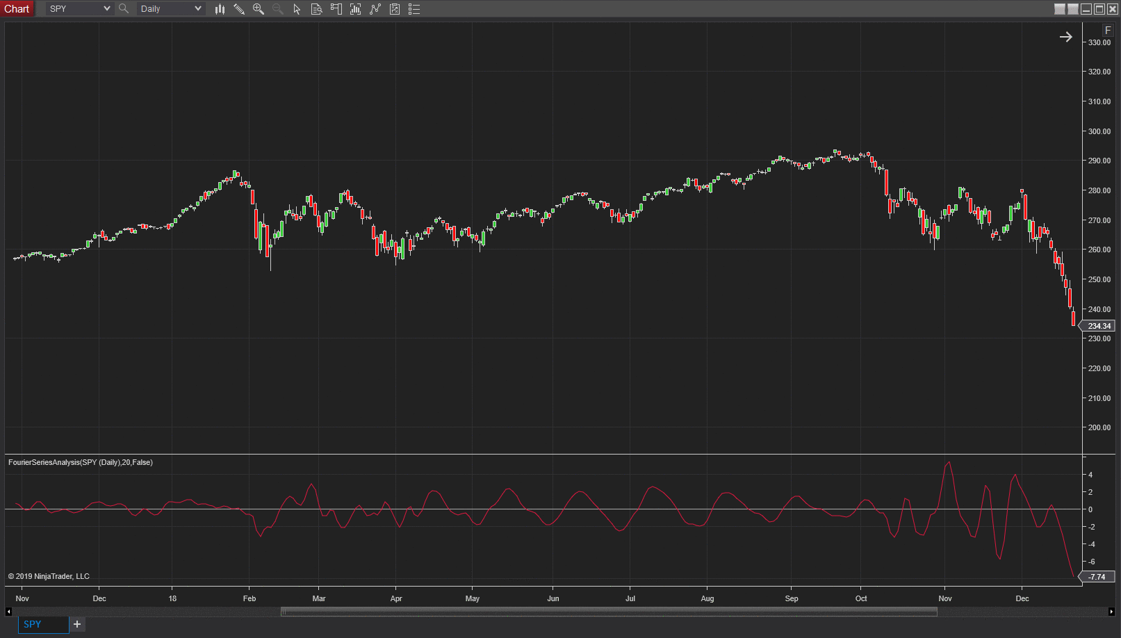
A sample chart implementing the indicator is shown in Figure 7.

FIGURE 7: NINJATRADER. This shows the FourierSeriesAnalysis indicator displayed on a daily SPY chart from November 2017 to December 2018.
—Raymond Deux & Chris Lauber
NinjaTrader, LLC
www.ninjatrader.com
BACK TO LIST

TRADE NAVIGATOR: JUNE 2019
In the article “Fourier Series Model Of The Market” in this issue, author John Ehlers describes a Fourier series indicator. Users of Trade Navigator can download this library in Trade Navigator.
To download this library, click on Trade Navigator’s telephone button (or use the pull-down menu and then click “update data”), select “download special file,” then click on the start button. You will then be guided through an upgrade of your Trade Navigator. If you are prompted to “reimport libraries,” please do so. This will import the new indicator into the software.
Once this update is complete, you can insert the Fourier series indicator onto a chart by opening the charting dropdown menu, selecting the add to chart command, then on the indicators tab, finding the Fourier series indicator, selecting it, then clicking on the add button. Repeat this procedure for additional indicators as well if you wish.
Users may contact our technical support staff by phone or by live chat if any assistance is needed in importing the library.
A chart displaying the indicator is shown in Figure 8.

FIGURE 8: TRADE NAVIGATOR. Here, the Fourier series indicator is displayed in the lower panel on a chart of SPY.
BACK TO LIST
MICROSOFT EXCEL: JUNE 2019
In his article in this issue, “Fourier Series Model Of The Market,” author John Ehlers presents a very interesting Fourier-based oscillator construct that maps very nicely to cyclic price swings while filtering out much of the higher-frequency cycle noise.
He then suggests that the trader can apply rate-of-change (ROC) logic to pinpoint the extreme high and low turning points of this Fourier-based oscillator and thus the underlying turning points of the price action. This is a good tool to suggest potential swing trading entry and exit points.
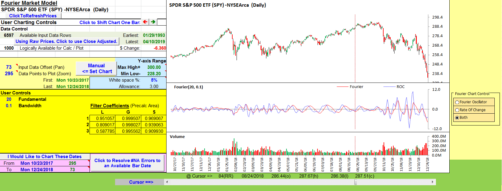
The Fourier oscillator (Figure 9) can also help differentiate trending periods from cycle-mode periods by way of the oscillator swing amplitudes.

FIGURE 9: EXCEL, FOURIER OSCILLATOR
This oscillator and the ROC crossover signals can be a great addition to any already-robust trading decision system but should not be used as a standalone system.
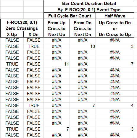
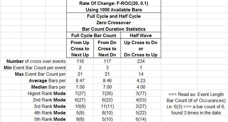
I got a little curious about this F-ROC signaling technique and Figures 10 and 11 show the simple statistics this spreadsheet collects.

FIGURE 10: EXCEL, BAR COUNT TO NEXT EVENT

FIGURE 11: EXCEL, SIMPLE EVENT-TYPE STATISTICS
The formulas in columns just to the right of the charts, which are shown in Figure 10, keep track of the number of bars until the next occurrence of the indicated F-ROC crossover types. Of particular interest, the half wave would be the duration of a long or short swing trade when based on F-ROC crossovers.
Figure 11 provides a couple of interesting bits. When using “20” as the fundamental cycle length for the Fourier construct, the F-ROC detected full cycle lengths, either up to up, or down to down, clustered around seven bars.
For swing traders, the half wave (long or short position duration) clusters around four bars.
Ehlers suggests 20 as a fundamental cycle length for these calculations, as that is roughly the number of trading days in a month.
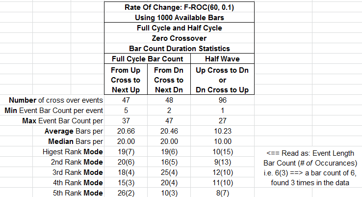
Just for grins, I thought to try 60 as an approximation of the number of trading days in a quarter.
One interesting result, seen in Figure 12, is that with the fundamental cycle length set to 60, the full cycle numbers cluster around 20 bars, similar to Ehlers’ observation for the trading length of a month.

FIGURE 12: EXCEL, STATISTICS FOR A FUNDAMENTAL CYCLE LENGTH OF 60
The spreadsheet file for this Traders’ Tip can be downloaded from Traders.com in the Traders’ Tips area. To successfully download it, follow these steps:
- Right-click on the Excel file link, then
- Select “save as” (or “save target as”) to place a copy of the spreadsheet file on your hard drive.
—Ron McAllister
Excel and VBA programmer
rpmac_xltt@sprynet.com
BACK TO LIST

AMIBROKER: JUNE 2019
In his article in this issue, “Fourier Series Model Of The Market,” John Ehlers presents a new Fourier series indicator that describes cyclic market activity to help swing traders develop trading strategy rules. Ready-to-use code is provided below.
// Fourier Series Analysis

Fundamental = 20;
Bandwidth = 0.1;
TWOPI = 2 * 3.1415926;

//compute filter coefficients
L1 = cos( TWOPI / Fundamental);
G1 = cos( Bandwidth*TWOPI / Fundamental);
S1 = 1 / G1 - sqrt(1 / (G1*G1) - 1);
L2 = cos(TWOPI / (Fundamental / 2));
G2 = cos(Bandwidth*TWOPI / (Fundamental / 2));
S2 = 1 / G2 - sqrt(1 / (G2*G2) - 1);
L3 = cos(TWOPI / (Fundamental / 3));
G3 = cos(Bandwidth*TWOPI / (Fundamental / 3));
S3 = 1 / G3 - sqrt(1 / (G3*G3) - 1);


// Fundamental Band-Pass
// 2nd order IIR
// IIR( array, b0,
//             a1, b1,
//             a2, b2 )
// aX - output (feedback) at X bar back
// bX - input at X bar back

BP1 = IIR( Close, 0.5*( 1 - S1 ),
                  L1*(1 + S1), 0,
                  -S1, - 0.5*( 1 - S1 ) );

// Fundamental Quadrature
Q1 = (Fundamental / TWOPI)*(BP1 - Ref(BP1, -1 ));

//Second Harmonic Band-Pass
BP2 = IIR( Close, 0.5*(1 - S2),
                  L2*(1 + S2), 0,
                  -S2, - 0.5*(1 - S2) );

//Second Harmonic Quadrature
Q2 = (Fundamental / TWOPI)*(BP2 - Ref( BP2, -1 ));

// Third Harmonic Band-Pass
BP3 = IIR( Close, 0.5*(1 - S3),
                  L3*(1 + S3), 0,
                  -S3, - 0.5*(1 - S3) );


//Third Harmonic  Quadrature
Q3 = (Fundamental / TWOPI)*(BP3 - Ref(BP3, -1) );

// Sum power of each harmonic at each bar over the Fundamental period
P1 = 0; P2 = 0; P3 = 0;
for( count = 0; count < Fundamental; count++ )
{
  b = Ref( BP1, -count ); q = Ref( Q1, -count );
  P1 += b * b + q * q;
  b = Ref( BP2, -count ); q = Ref( Q2, -count );
  P2 += b * b + q * q;
  b = Ref( BP3, -count ); q = Ref( Q3, -count );
  P3 += b * b + q * q;
}

// Add the three harmonics together using their relative amplitudes
Wave = BP1 + sqrt(P2 / P1)*BP2 + sqrt(P3 / P1)*BP3;

Plot(Wave, "Wave", colorRed );

// Optional cyclic trading signal
// Rate of change crosses zero at cyclic turning points
rocc = (Fundamental / 12.57)*(Wave - Ref(Wave, -2));
// Plot(rocc, "Rate of change crosses zero", colorBlue);
A sample chart is shown in Figure 13.

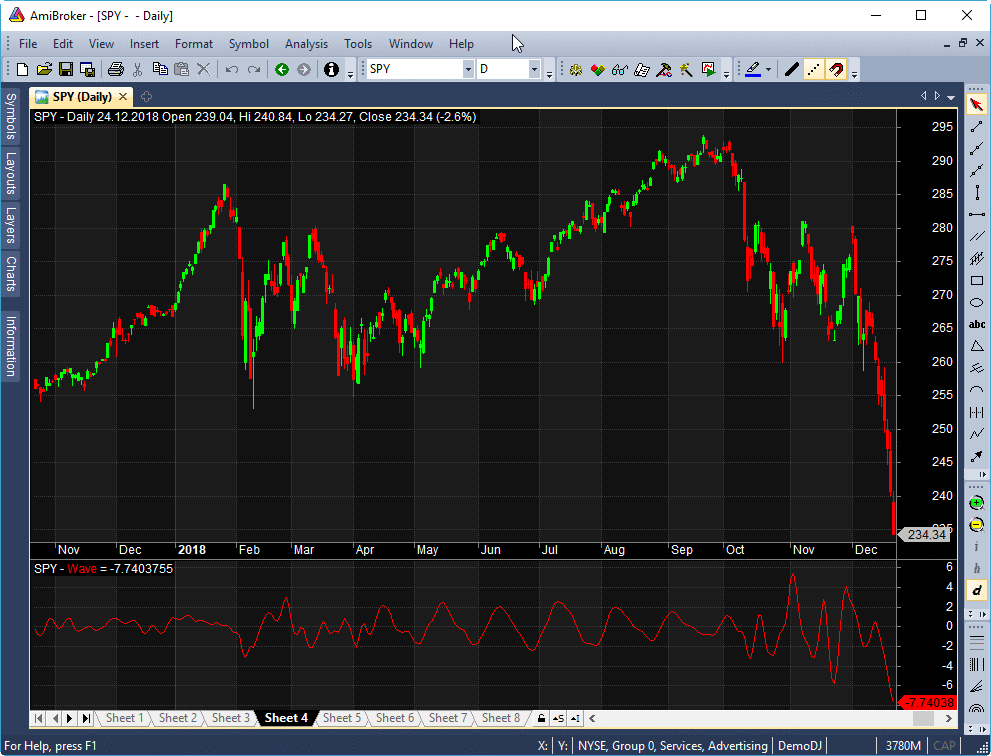
FIGURE 13: AMIBROKER. This daily chart of SPY with the Fourier series indicator (wave) in the lower pane replicates the chart from the referenced article in this issue.
—Tomasz Janeczko, AmiBroker.com
www.amibroker.com
BACK TO LIST

TRADERSSTUDIO: JUNE 2019
The importable TradersStudio files based on John Ehlers’ article in this issue, “Fourier Series Model of The Market,” can be obtained on request via email to info@TradersEdgeSystems.com. The code is also available at Traders.com in the Traders’ Tips area.
The author did not provide complete code for a trading system. The code I am supplying may not be what the author intended. It only seems to work when traded without commissions or slippage so additional work is needed to convert this to a real-world trading system.
'Fourier Series Model of The Market
'Author: John F. Ehlers, TASC Jun 2019
'Coded by: Richard Denning, 4/16/2019
'www.TradersEdgeSystems.com

'Compute filter coefficients once
Function WAVE(Fundamental,Bandwidth)
  'Fundamental = 20
    Dim G1 As BarArray
    Dim S1 As BarArray
    Dim L1 As BarArray
    Dim BP1 As BarArray
    Dim Q1 As BarArray
    Dim P1 As BarArray
    Dim G2 As BarArray
    Dim S2 As BarArray
    Dim L2 As BarArray
    Dim BP2 As BarArray
    Dim Q2 As BarArray
    Dim P2 As BarArray
    Dim G3 As BarArray
    Dim S3 As BarArray
    Dim L3 As BarArray
    Dim BP3 As BarArray
    Dim Q3 As BarArray
    Dim P3 As BarArray
    Dim count As BarArray

   If CurrentBar = 1 Then
        L1 = TStation_Cosine(360 / Fundamental)
        G1 = TStation_Cosine(Bandwidth*360 / Fundamental)
        S1 = 1 / G1 - Sqr(1 / (G1*G1) - 1)
        L2 = TStation_Cosine(360 / (Fundamental / 2))
        G2 = TStation_Cosine(Bandwidth*360 / (Fundamental / 2))
        S2 = 1 / G2 - Sqr(1 / (G2*G2) - 1)
        L3 = TStation_Cosine(360 / (Fundamental / 3))
        G3 = TStation_Cosine(Bandwidth*360 / (Fundamental / 3))
        S3 = 1 / G3 - Sqr(1 / (G3*G3) - 1)
   End If

'Fundamental Band-Pass
    BP1 = .5*(1 - S1)*(Close - Close[2]) + L1*(1 + S1)*BP1[1] - S1*BP1[2]

'Fundamental Quadrature
    Q1 = (Fundamental / 6.28)*(BP1 - BP1[1])

'Second Harmonic Band-Pass
    BP2 = .5*(1 - S2)*(Close - Close[2]) + L2*(1 + S2)*BP2[1] - S2*BP2[2]

'Second Harmonic Quadrature
    Q2 = (Fundamental / 6.28)*(BP2 - BP2[1])

'Thrid Harmonic Band-Pass
    BP3 = .5*(1 - S3)*(Close - Close[2]) + L3*(1 + S3)*BP3[1] - S3*BP3[2]
    Q3 = (Fundamental / 6.28)*(BP3 - BP3[1])

'Sum power of each harmonic at each bar over the Fundamental period
    P1 = 0
    P2 = 0
    P3 = 0
    For count = 0 To Fundamental - 1
        P1 = P1 + BP1[count]*BP1[count] + Q1[count]*Q1[count]
        P2 = P2 + BP2[count]*BP2[count] + Q2[count]*Q2[count]
        P3 = P3 + BP3[count]*BP3[count] + Q3[count]*Q3[count]
    Next

'Add the three harmonics together using their relative amplitudes
    If P1 <> 0 Then
        WAVE = BP1 + Sqr(P2 / P1)*BP2 + Sqr(P3 / P1)*BP3
    End If
'Print FormatDateTime(Date)," P1 ",P1," WAVE ",wave
End Function
'----------------------------------------------------------------------
Function TSTATION_COSINE(TSdegrees)
TSTATION_COSINE = Cos(DegToRad(TSdegrees))
End Function
'----------------------------------------------------------------------
'Code to plot indicator
Sub WAVE_IND(FundamentalLen,Bandwidth)
Dim theWAVE As BarArray
theWAVE = WAVE(FundamentalLen,Bandwidth)
plot1(theWAVE)
'-----------------------------------------------------------------------
'Optional cyclic trading signal
'Rate Of change crosses zero at cyclic turning points
Sub WAVE_SYS(FundamentalLen,Bandwidth)
Dim theWAVE As BarArray
Dim theROC As BarArray
theWAVE = WAVE(FundamentalLen,Bandwidth)
theROC = (FundamentalLen / 12.57)*(theWAVE - theWAVE[2])
If theROC[1] >= 0 And theROC < 0 Then Buy("LE",1,0,Market,Day)
If theROC[1] <= 0 And theROC > 0 Then ExitLong("LX","",1,0,Market,Day)
If theROC[1] <= 0 And theROC > 0 Then Sell("SE",1,0,Market,Day)
If theROC[1] >= 0 And theROC < 0 Then ExitShort("SX","",1,0,Market,Day)
End Sub
'------------------------------------------------------------------------
End Sub
—Richard Denning
info@TradersEdgeSystems.com
for AIQ Systems
BACK TO LIST
Originally published in the June 2019 issue of
Technical Analysis of STOCKS & COMMODITIES magazine.
All rights reserved. © Copyright 2019, Technical Analysis, Inc.
