TRADERS’ TIPS
June 2021

For this month’s Traders’ Tips, the focus is John Ehlers’ article in this issue, “Creating More Robust Trading Strategies With The FM Demodulator.” Here, we present the June 2021 Traders’ Tips code with possible implementations in various software.
You can right-click on any chart to open it in a new tab or window and view it at it’s originally supplied size, often much larger than the version printed in the magazine.
The Traders’ Tips section is provided to help the reader implement a selected technique from an article in this issue or another recent issue. The entries here are contributed by software developers or programmers for software that is capable of customization.

TRADESTATION: JUNE 2021
In his article “Creating More Robust Trading Strategies With The FM Demodulator” in this issue, author John Ehlers builds upon his article in last month’s issue, which discussed using FM demodulation to identify and isolate volatility components from the timing components found in market data.
His article in this issue introduces the use of FM demodulation in strategies to reduce the variation of parameter settings as the data changes. The author states in his article that the main advantage of incorporating the FM discriminator into a strategy is that it can improve a strategy’s robustness over time.
Provided here is some EasyLanguage code for the two strategies found in the article—one being a simple example strategy and the other, a simple strategy that includes FM demodulation to help illustrate the difference.
Strategy:  _TASC_JUN_2021_Simple Strategy
// TASC JUN 2021
// Creating More Robust Trading Strategies With The FM
// Demodulator
// (c) 2013 - 2021 John F. Ehlers
// Simple strategy

inputs:
	SigPeriod( 8 ),
	ROCPeriod( 1 );

variables:
	Deriv( 0 ),
	Z3( 0 ),
	Signal( 0 ),
	ROC( 0 );

// derivative of the price wave
Deriv = Close - Close[2];

// zeros at Nyquist and 2 * Nyquist,
// i.e. Z3 = (1 + Z^-1)*(1 + Z^-2) to integrate
// derivative
Z3 = Deriv + Deriv[1] + Deriv[2] + Deriv[3];

// smooth Z3 for trading signal
Signal = Average( Z3, SigPeriod );

// use Rate of Change to identify entry point
ROC = Signal - Signal[ROCPeriod];

if ROC crosses over 0 then
	Buy next bar on Open;

if Signal crosses under 0 then
	Sell next bar on Open;


Strategy:  TASC JUN 2021 Strategy With FM Demodulator
// TASC JUN 2021
// Creating More Robust Trading Strategies With The FM
// Demodulator
// (c) 2013 - 2021 John F. Ehlers
// Simple strategy with FM demodulator

inputs:
	SigPeriod( 22 ),
	ROCPeriod( 10 );

variables:
	Deriv( 0 ),
	RMS( 0 ),
	count( 0 ),
	Clip( 0 ),
	Z3( 0 ),
	Signal( 0 ),
	ROC( 0 );

// derivative of the price wave
Deriv = Close - Close[2];

// normalize Degap to half RMS and hard limit at +/- 1
RMS = 0;

for count = 0 to 49
begin
	RMS = RMS + Deriv[count] * Deriv[count];
end;

if RMS <> 0 then
	Clip = 2 * Deriv / SquareRoot( RMS / 50 );

if Clip > 1 then
	Clip = 1;

if Clip < -1 then
	Clip = -1;

// zeros at Nyquist and 2*Nyquist,
// i.e. Z3 = (1 + Z^-1)*(1 + Z^-2) to integrate
// derivative
Z3 = Clip + Clip [1] + Clip [2] + Clip [3];

// smooth Z2 for trading signal
Signal = Average( Z3, SigPeriod );

// use Rate of Change to identify entry point
ROC = Signal - Signal[ROCPeriod];

if ROC crosses over 0 then
	Buy next bar on Open;

if Signal crosses under 0 then
	Sell next bar on Open;
To download the EasyLanguage code for TradeStation 10, please visit our TradeStation and EasyLanguage support forum. The files for this article can be found here: https://community.tradestation.com/discussions/Topic.aspx?Topic_ID=190289
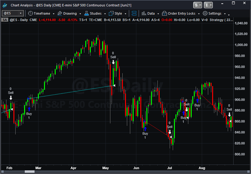
A sample chart is shown in Figure 1.

FIGURE 1: TRADESTATION. This daily chart of the S&P 500 emini futures continuous contract shows the demodulated strategy applied.
This article is for informational purposes. No type of trading or investment recommendation, advice, or strategy is being made, given, or in any manner provided by TradeStation Securities or its affiliates.
—Chris Imhof
TradeStation Securities, Inc.
www.TradeStation.com
BACK TO LIST

THINKORSWIM: JUNE 2021
We have put together a strategy based on the article by John Ehlers in this issue titled “Creating More Robust Trading Strategies With The FM Demodulator.” We built the strategy referenced by using our proprietary scripting language, thinkscript. To ease the loading process, simply click on https://tos.mx/DOh8z2x or enter it into the address in setup→open shared item from within thinkorswim and then choose view thinkScript strategy and name it “SimpleROC” or whatever name you like and can identify it by. You can then add the strategy to your charts from the edit studies menu, then click on the strategy tab from within the charts tab.
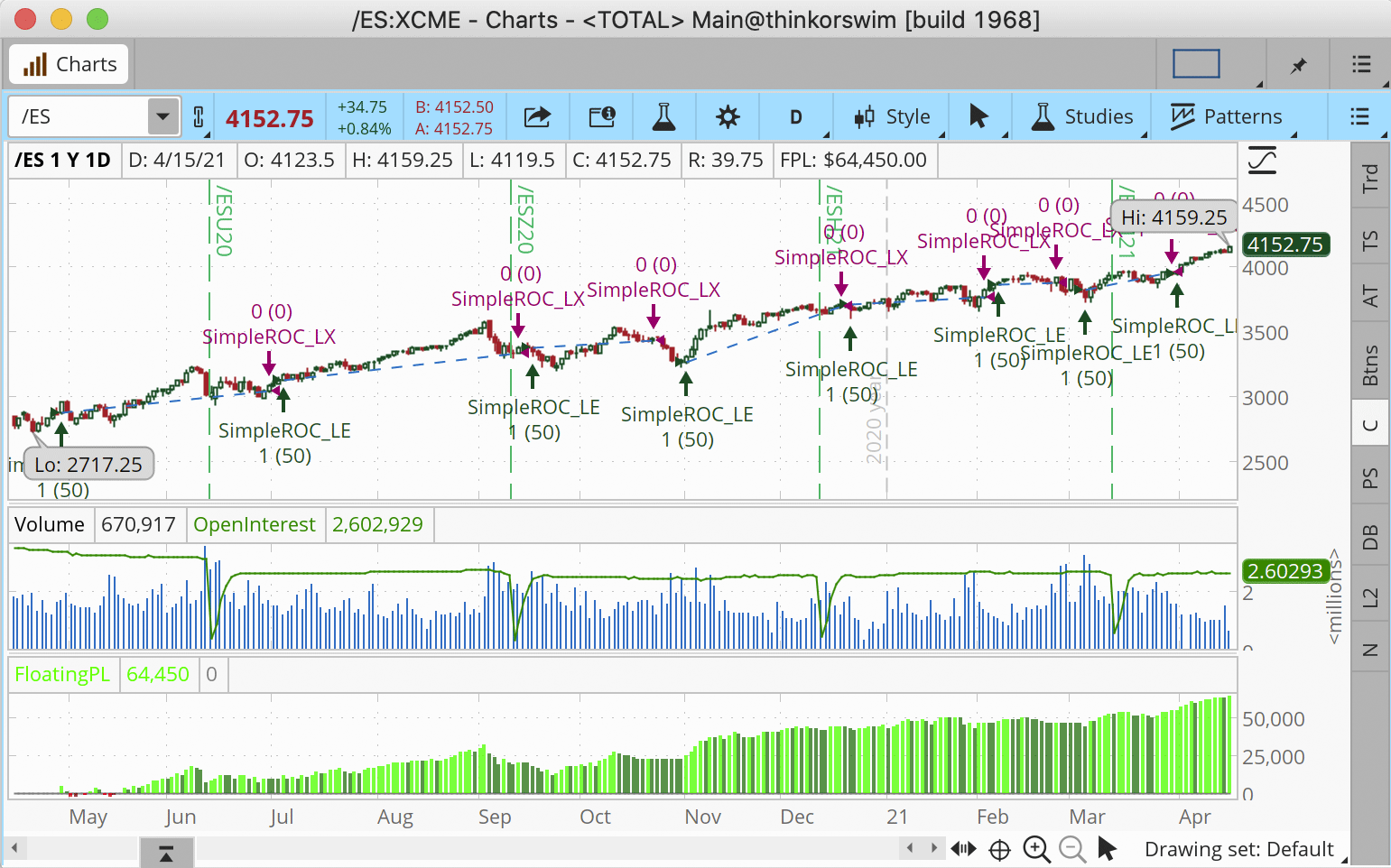
The chart in Figure 2 contains the simple ROC strategy applied to a daily chart of emini S&P 500 index futures with the FM demodulator enabled. It is controlled via the correspondent “use FM demodulator” input to enable/disable FM demodulator. The FM demodulator is enabled by default. Please reference John Ehlers’ article for more details.

FIGURE 2: THINKORSWIM. The referenced study is shown on a chart of emini S&P 500 index futures with the FM demodulator enabled.
—thinkorswim
A division of TD Ameritrade, Inc.
www.thinkorswim.com
BACK TO LIST

eSIGNAL: JUNE 2021
For this month’s Traders’ Tip, we’ve provided the study “SimpleStrategies.efs” based on the article by John Ehlers in this issue, “Creating More Robust Trading Strategies With The FM Demodulator.” The study helps in creating simpler and more robust strategies.
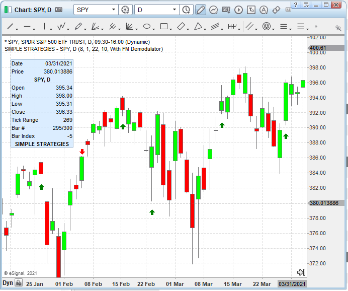
The study contains formula parameters that may be configured through the edit chart window (right-click on the chart and select “edit chart”). A sample chart is shown in Figure 3.

FIGURE 3: eSIGNAL. Here is an example of the study plotted on a daily chart of SPY.
To discuss this study or download a complete copy of the formula code, please visit the EFS library discussion board forum under the forums link from the support menu at www.esignal.com or visit our EFS KnowledgeBase at https://www.esignal.com/support/kb/efs/. The eSignal formula script (EFS) is also available here:
/**********************************
Provided By:
Copyright 2019 Intercontinental Exchange, Inc. All Rights Reserved.
eSignal is a service mark and/or a registered service mark of Intercontinental Exchange, Inc.
in the United States and/or other countries. This sample eSignal Formula Script (EFS)
is for educational purposes only.
Intercontinental Exchange, Inc. reserves the right to modify and overwrite this EFS file with each new release.

Description:
    Creating More Robust Trading Strategies With The FM Demodulator
    by John F. Ehlers


Version:            1.00  04/08/2021

Formula Parameters:                    Default:
SigPeriod                              8
ROCPeriod                              1
SigPeriod2                             22
ROCPeriod2                             10

Notes:
The related article is copyrighted material. If you are not a subscriber
of Stocks & Commodities, please visit www.traders.com.

**********************************/
var fpArray = new Array();
var bInit = false;

function preMain() {
    setStudyTitle("Simple Strategies");
    setPriceStudy(true);

    var x=0;
    fpArray[x] = new FunctionParameter("SigPeriod", FunctionParameter.NUMBER);
	with(fpArray[x++]){
        setLowerLimit(1);
        setDefault(8);
    }
    fpArray[x] = new FunctionParameter("ROCPeriod", FunctionParameter.NUMBER);
	with(fpArray[x++]){
        setLowerLimit(1);
        setDefault(1);
    }
     fpArray[x] = new FunctionParameter("SigPeriod2", FunctionParameter.NUMBER);
	with(fpArray[x++]){
        setName("SigPeriod Demodulator");
        setLowerLimit(1);
        setDefault(22);
    }
    fpArray[x] = new FunctionParameter("ROCPeriod2", FunctionParameter.NUMBER);
	with(fpArray[x++]){
        setName("ROCPeriod Demodulator");
        setLowerLimit(1);
        setDefault(10);
    }
    fpArray[x] = new FunctionParameter("Type", FunctionParameter.STRING);
	with(fpArray[x++]){
        setName("Type");
        addOption("Standard");
        addOption("With FM Demodulator");
        setDefault("Standard");
    }
}

var bVersion = null;
var xClose = null;
var xOpen = null;
var xDeriv = null;
var xZ3 = null;
var xSignal = null;
var xROC = null;


function main(SigPeriod, ROCPeriod, SigPeriod2, ROCPeriod2, Type) {
    if (bVersion == null) bVersion = verify();
    if (bVersion == false) return;

    if ( bInit == false ) {
        xClose = close();
        xHigh = high();
        xLow = low();
        xDeriv = efsInternal("Calc_Deriv", xClose);
        if (Type=="Standard"){
            xZ3 = efsInternal("Calc_z3", xDeriv);
            xSignal = sma(SigPeriod, xZ3);
            xROC = roc(ROCPeriod, xSignal);
        }
        else {
            xClip = efsInternal("Calc_clip", xDeriv);
            xZ3 = efsInternal("Calc_z3", xClip);
            xSignal = sma(SigPeriod2, xZ3);
            xROC = roc(ROCPeriod2, xSignal);
        }

        bInit = true;
    }

    if (xROC.getValue(-2) < 0 && xROC.getValue(-1) > 0) {
        drawShapeRelative(0, xLow.getValue(0) - getMinTick()*100, Shape.UPARROW, null, Color.green, Shape.ONTOP | Shape.TOP, "buy" + getCurrentBarCount());
    }
    if (xSignal.getValue(-2) > 0 && xSignal.getValue(-1) < 0){
        drawShapeRelative(0, xHigh.getValue(0) + getMinTick()*100, Shape.DOWNARROW, null, Color.red, Shape.ONTOP  | Shape.TOP, "sell" + getCurrentBarCount());
    }

    return;
}

function Calc_clip(xDeriv){
    var RMS = 0;
    var ret = 0;
    for (var i = 0; i <=49; i++){
        RMS = RMS + xDeriv.getValue(-i) * xDeriv.getValue(-i);
    }
    if (RMS != 0) ret = 2 * xDeriv.getValue(0) / Math.sqrt(RMS/50);
    if (ret > 1) ret = 1;
    if (ret < -1) ret = -1;

    return ret;
}

function Calc_z3(xDeriv){
    var ret = 0;
    ret = xDeriv.getValue(0) + xDeriv.getValue(-1) + xDeriv.getValue(-2) + xDeriv.getValue(-3);
    return ret;
}

function Calc_Deriv(xClose){
    var ret = 0;
    ret = xClose.getValue(0) - xClose.getValue(-2);
    return ret;
}

function verify(){
    var b = false;
    if (getBuildNumber() < 779){

        drawTextAbsolute(5, 35, "This study requires version 10.6 or later.",
            Color.white, Color.blue, Text.RELATIVETOBOTTOM|Text.RELATIVETOLEFT|Text.BOLD|Text.LEFT,
            null, 13, "error");
        drawTextAbsolute(5, 20, "Click HERE to upgrade.@URL=https://www.esignal.com/download/default.asp",
            Color.white, Color.blue, Text.RELATIVETOBOTTOM|Text.RELATIVETOLEFT|Text.BOLD|Text.LEFT,
            null, 13, "upgrade");
        return b;
    }
    else
        b = true;

    return b;
}
—Eric Lippert
eSignal, an Interactive Data company
800 779-6555, www.eSignal.com
BACK TO LIST

WEALTH-LAB.COM: JUNE 2021
In his article in this issue, “Creating More Robust Trading Strategies With The FM Demodulator,” John Ehlers presents an example strategy to demonstrate application of the FM demodulator indicator (for educational purposes only). Here is the code for implementing it in Wealth-Lab.
using WealthLab.Backtest;
using System;
using WealthLab.Core;
using WealthLab.Indicators;
using System.Drawing;
using System.Collections.Generic;

namespace TASCStrategies
{
	public class TASC202106 : UserStrategyBase
	{
		public override void Initialize(BarHistory bars)
		{
			roc = new TimeSeries( bars.DateTimes, 0);
			signal = new TimeSeries( bars.DateTimes, 0);
			clip = new TimeSeries( bars.DateTimes, 0);
			Z3 = new TimeSeries( bars.DateTimes, 0);
			RMS = new TimeSeries( bars.DateTimes, 0);

			/* Derivative of the price wave */
			var Deriv = bars.Close - (bars.Close >> 2);
			Deriv[0] = Deriv[1] = 0;

			for (int bar = 0; bar < bars.Count; bar++)
			{
				if (bar >= period)
				{
					for (int count = 0; count < period - 1; count++)
					{
						if (bar > period)
							rms += Math.Pow(Deriv[bar - count], 2);
					}

					RMS[bar] = rms;

					double _clip = 0;
					if (RMS[bar] != 0)
						_clip = 2 * Deriv[bar] / Math.Sqrt(RMS[bar] / 50);
					if (_clip > 1) _clip = 1;
					if (_clip < -1) _clip = -1;
					clip[bar] = _clip;

					/* zeros at Nyquist and 2*Nyquist, i.e. Z3 = (1 + Z^-1)*(1 + Z^-2) to integrate derivative */
					Z3[bar] = clip[bar] + clip[bar - 1] + clip[bar - 2] + clip[bar - 3];
				}
			}

			/* Smooth Z2 for trading signal */
			signal = SMA.Series(Z3, SigPeriod);
			/* Use Rate of Change to identify entry point */
			roc = signal - (signal >>ROCPeriod);

			PlotTimeSeries( signal, "Signal", "FMD", Color.Red);
			PlotTimeSeries( roc, "RoC", "FMD");
			DrawHorzLine( 0, Color.Violet, 2, LineStyles.Dashed, "FMD");

			StartIndex = Math.Max(ROCPeriod, Math.Max(SigPeriod, period));
		}

		public override void Execute(BarHistory bars, int idx)
		{
			if (!HasOpenPosition(bars, PositionType.Long))
			{
				/* If ROC Crosses Over 0 Then Buy Next Bar on Open;*/
				if (roc.CrossesOver(0, idx))
					PlaceTrade( bars, TransactionType.Buy, OrderType.Market);
			}
			else
			{
				/* If Signal Crosses Under 0 Then Sell Next Bar on Open; */
				if (signal.CrossesUnder(0, idx))
					ClosePosition( LastPosition, OrderType.Market);
			}
		}

		/* declare private variables below */
		TimeSeries roc, signal, clip, Z3, RMS;
		int SigPeriod = 22, ROCPeriod = 10, period = 49; /* Normalize Degap to half RMS and hard limit at +/- 1 */
		double rms = 0;
	}
}

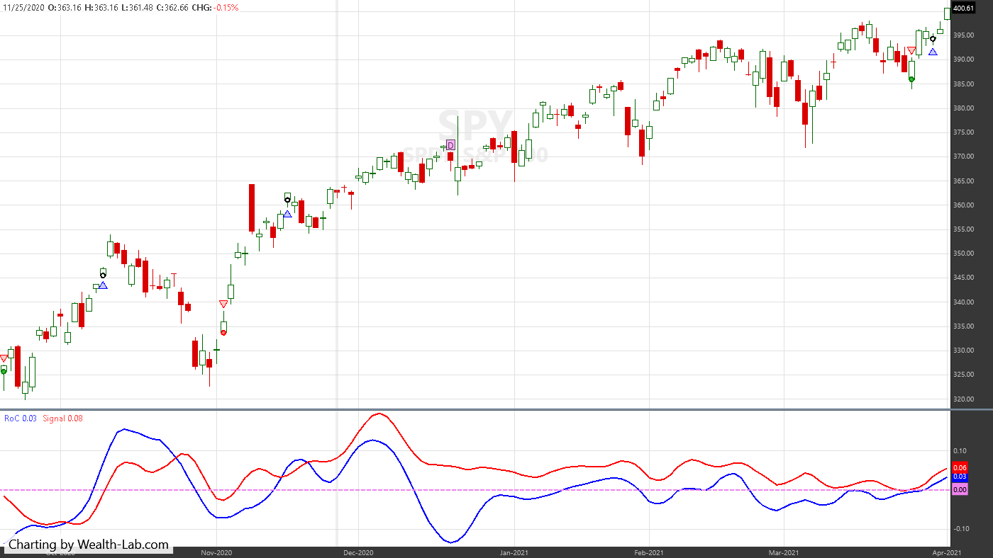
FIGURE 4: WEALTH-LAB. Sample trades are shown on a chart of SPY. The adjusted ROC and signal indicators are plotted in the bottom pane.
—Gene Geren (Eugene)
Wealth-Lab team
www.wealth-lab.com
BACK TO LIST

NINJATRADER: JUNE 2021
The simple strategy and simple clip strategy, as discussed in John Ehlers’ article in this issue, “Creating More Robust Trading Strategies With The FM Demodulator,” are available for download at the following links for NinjaTrader 8 and for NinjaTrader 7:
Once the file is downloaded, you can import the strategies in NinjaTader 8 from within the control center by selecting Tools → Import → NinjaScript Add-On and then selecting the downloaded file for NinjaTrader 8. To import into NinjaTrader 7, from within the control center window, select the menu File → Utilities → Import NinjaScript and select the downloaded file.
You can review the source code for both strategies in NinjaTrader 8 by selecting the menu New → NinjaScript Editor → Strategies from within the control center window and selecting the SimpleStrategy or SimpleClip file. You can review the strategies’ source code in NinjaTrader 7 by selecting the menu Tools → Edit NinjaScript → Strategy from within the control center window and selecting the SimpleStrategy or SimpleClip file.
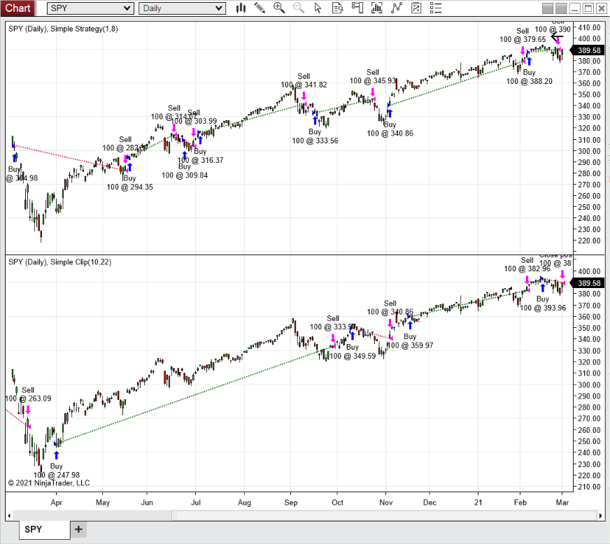
A sample chart displaying the strategies is shown in Figure 5.

FIGURE 5: NINJATRADER. The daily chart shows the SPDR S&P 500 ETF (SPY) with the simple strategy in the upper pane and the simple clip strategy in the bottom pane from March 2020 through February 2021.
NinjaScript uses compiled DLLs that run native, not interpreted, to provide you with the highest performance possible.
—Kate Windheuser
NinjaTrader, LLC
www.ninjatrader.com
BACK TO LIST

NEUROSHELL TRADER: JUNE 2021
The simple strategy given to demonstrate implementation of the FM demodulator that is described by John Ehlers in his article in this issue can be easily implemented with a few of NeuroShell Trader’s 800+ indicators and trading strategy wizard. First, select new indicator from the insert menu and use the indicator wizard to create the following indicators:
Signal	Avg(Sum(Momentum(Close,2),4),8)

FMSignal	Avg( Sum( Max2( -1, Min2( Divide( Mul2( 2, Momentum( Close, 2)), SqrRt( Divide( Sum( Mul2( Momentum( Close, 2), Momentum( Close, 2)), 50), 50))), 1)), 4), 22)
To implement the simple strategy, select new trading strategy from the insert menu and enter the following in the appropriate locations of the trading strategy wizard:
BUY LONG CONDITIONS: [All of which must be true]
     CrossAbove( Momentum( Signal, 1), 0)
SELL LONG CONDITIONS: [All of which must be true]
     CrossBelow( Signal,  0)
To implement the FM demodulator strategy, select new trading strategy from the insert menu and enter the following in the appropriate locations of the trading strategy wizard:
BUY LONG CONDITIONS: [All of which must be true]
     CrossAbove(Momentum( FMSignal, 10 ), 0)
SELL LONG CONDITIONS: [All of which must be true]
     CrossBelow( FMSignal, 0)
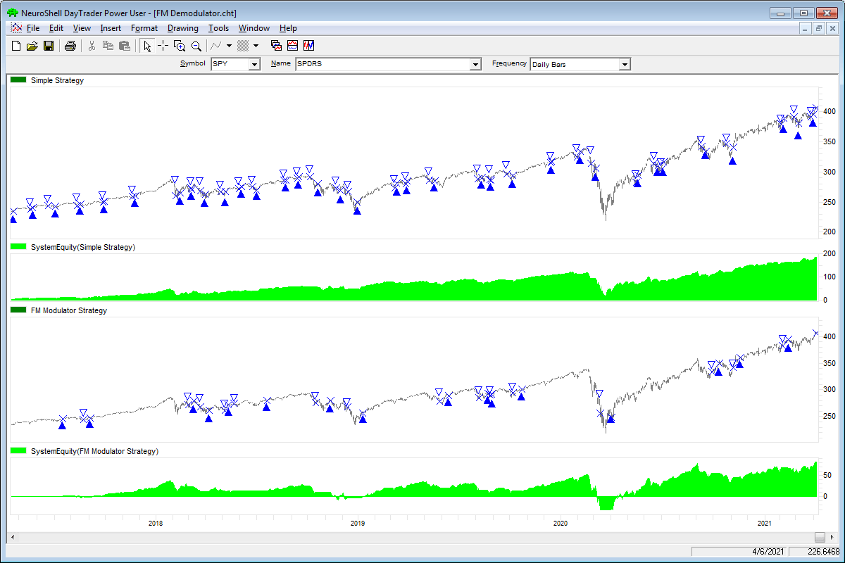
Figure 6 shows a chart of the example simple strategy with and without the FM demodulator applied to SPY.

FIGURE 6: NEUROSHELL TRADER. This NeuroShell Trader chart displays an example of the simple strategy with and without the FM demodulator applied to SPY.
NeuroShell Trader users can go to the Stocks & Commodities section of the NeuroShell Trader free technical support website to download a copy of this or any previous Traders’ Tips.
—Ward Systems Group, Inc.
sales@wardsystems.com
www.neuroshell.com
BACK TO LIST

OPTUMA: JUNE 2021
Here is a formula for Optuma for replicating the simple strategy that is given in John Ehlers’ article in this issue for the purposes of illustrating the use of incorporating the FM demodulator in a strategy.
Simple Strategy:
$SigPeriod = 8;
$ROCPeriod = 1;
Deriv = CLOSE()-CLOSE()[2];
Z3 = Deriv + Deriv[1] + Deriv[2] + Deriv[3];
Signal= MA(Z3, BARS=$SigPeriod, CALC=Close);
ROC1 = Signal - OFFSET(Signal, OFFSET=$ROCPeriod);
//Buy Signal;
ROC1 CrossesAbove 0
//Sell Signal;
//ROC1 CrossesBelow 0
Simple with FM Demodulator:
$SigPeriod = 22;
$ROCPeriod = 10;
Deriv = CLOSE()-CLOSE()[2];
Deriv2 = Deriv * Deriv;
RMS=ACC(Deriv2, RANGE=Look Back Period, BARS=50);
Clip = (2*Deriv) / SQRT(RMS / 50);
Z3 = Clip + Clip[1] + Clip[2] + Clip[3];
Signal= MA(Z3, BARS=$SigPeriod, CALC=Close);
ROC1 = Signal - OFFSET(Signal, OFFSET=$ROCPeriod);
//Buy Signal;
ROC1 CrossesAbove 0
//Sell Signal;
//ROC1 CrossesBelow 0
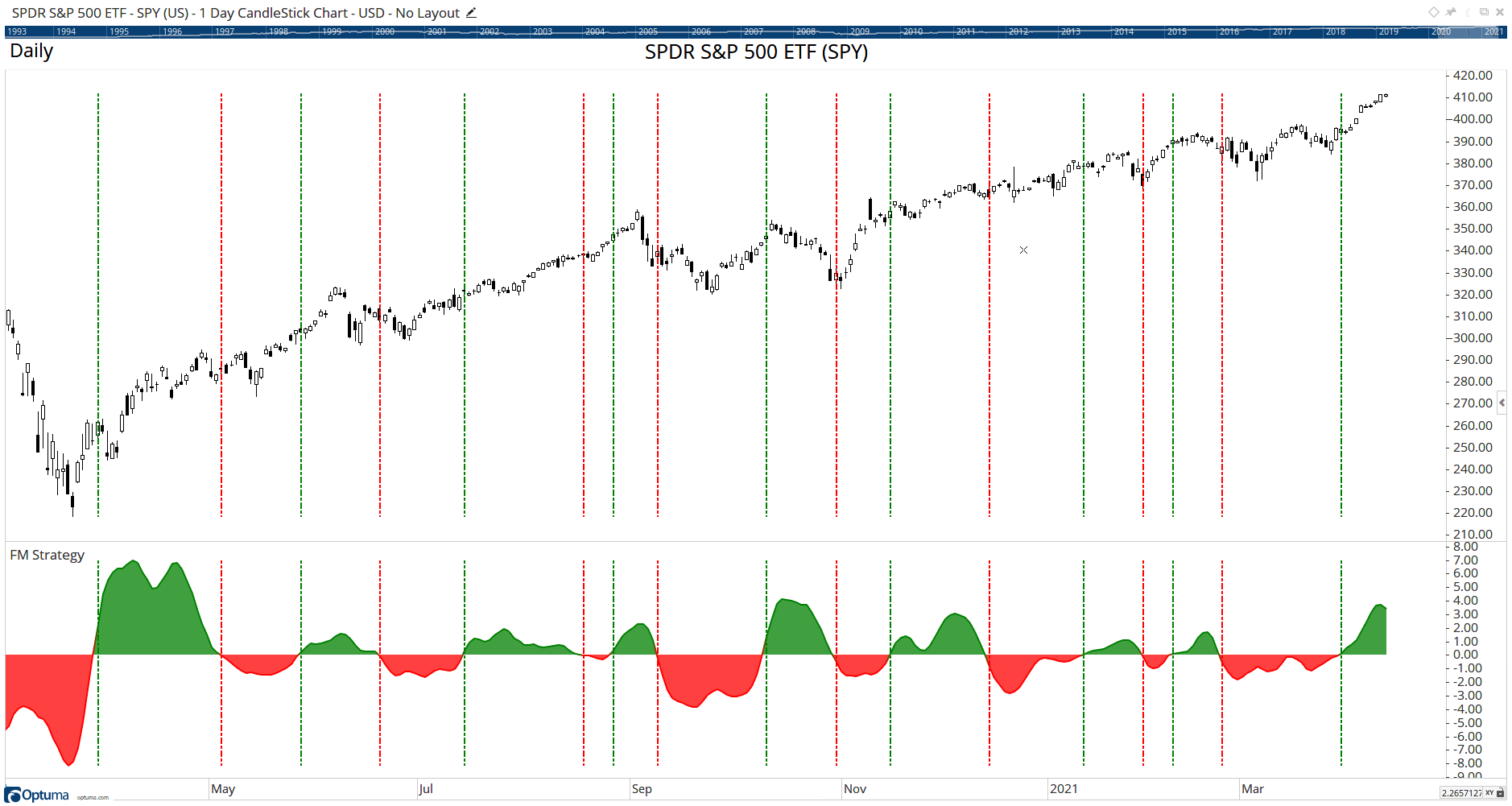
Figure 7 shows the example strategy on a chart. The green vertical lines show the buy signal, with red for the sells.

FIGURE 7: OPTUMA. The chart displays the simple strategy with the FM demodulator. The green vertical lines show the buy signal, with red for the sells.
—support@optuma.com
BACK TO LIST

TRADERSSTUDIO: JUNE 2021
The importable TradersStudio file for John Ehlers’ article, “Creating More Robust Trading Strategies With The FM Demodulator,” can be obtained on request via email to info@TradersEdgeSystems.com. The code is also shown below.
'Simple
'(c) 2013 - 2021 John F. Ehlers
Sub EHLERS_SIMPLE(SigPeriod, ROCPeriod)

    Dim Deriv As BarArray
    Dim Z3 As BarArray
    Dim Signal As BarArray
    Dim theROC As BarArray

    If BarNumber=FirstBar Then
        'SigPeriod = 8
        'ROCPeriod = 1
        Deriv = 0
        Z3 = 0
        Signal = 0
        theROC = 0
    End If

'Derivative of the price wave
    Deriv = Close - Close[2]
'zeros at Nyquist and 2*Nyquist,
'   i.e. Z3 = (1 + Z^-1)*(1 + Z^-2) to integrate derivative
    Z3 = Deriv + Deriv[1] + Deriv[2] + Deriv[3]
'Smooth Z3 for trading signal
    Signal = Average(Z3, SigPeriod)
'Use Rate of Change to identify entry point
    theROC = Signal - Signal[ROCPeriod]
    If CrossesOver(theROC, 0) Then
        Buy("", 1, 0, Market, Day)
    End If
    If CrossesUnder(Signal, 0) Then
        ExitLong("", "", 1, 0, Market, Day)
    End If
End Sub
'---------------------------------------------
'Simple Clip
'(c) 2013 - 2021 John F. Ehlers
Sub EHLERS_SIMPLE_CLIP(SigPeriod, ROCPeriod)

    Dim Deriv As BarArray
    Dim RMS As BarArray
    Dim count As BarArray
    Dim Clip As BarArray
    Dim Z3 As BarArray
    Dim Signal As BarArray
    Dim theROC As BarArray

    If BarNumber=FirstBar Then
        'SigPeriod = 22
        'ROCPeriod = 10
        Deriv = 0
        RMS = 0
        count = 0
        Clip = 0
        Z3 = 0
        Signal = 0
        theROC = 0
    End If

'Derivative of the price wave
    Deriv = Close - Close[2]
'Normalize Degap to half RMS and hard limit at +/- 1
    RMS = 0
    For count = 0 To 49
        RMS = RMS + Deriv [count]*Deriv [count]
    Next
    If RMS <> 0 Then
        Clip = 2*Deriv / Sqr(RMS / 50)
    End If
    If Clip > 1 Then
        Clip = 1
    End If
    If Clip < -1 Then
        Clip = -1
    End If
    Z3 = Clip + Clip [1] + Clip [2] + Clip [3]
'Smooth Z2 for trading signal
Signal = Average(Z3, SigPeriod)
'Use Rate of Change to identify entry point
    theROC = Signal - Signal[ROCPeriod]
    If CrossesOver(theROC, 0) Then
        Buy("LE", 1, 0, Market, Day)
    End If
    If CrossesUnder(Signal, 0) Then
        ExitLong("LX", "", 1, 0, Market, Day)
    End If
End Sub
'----------------------------------------------
Code for the Ehlers_Simple and Ehlers_Simple_Clip System is provided in the system code “EHLERS_SIMPLE” and “EHLERS_SIMPLE_CLIP.”
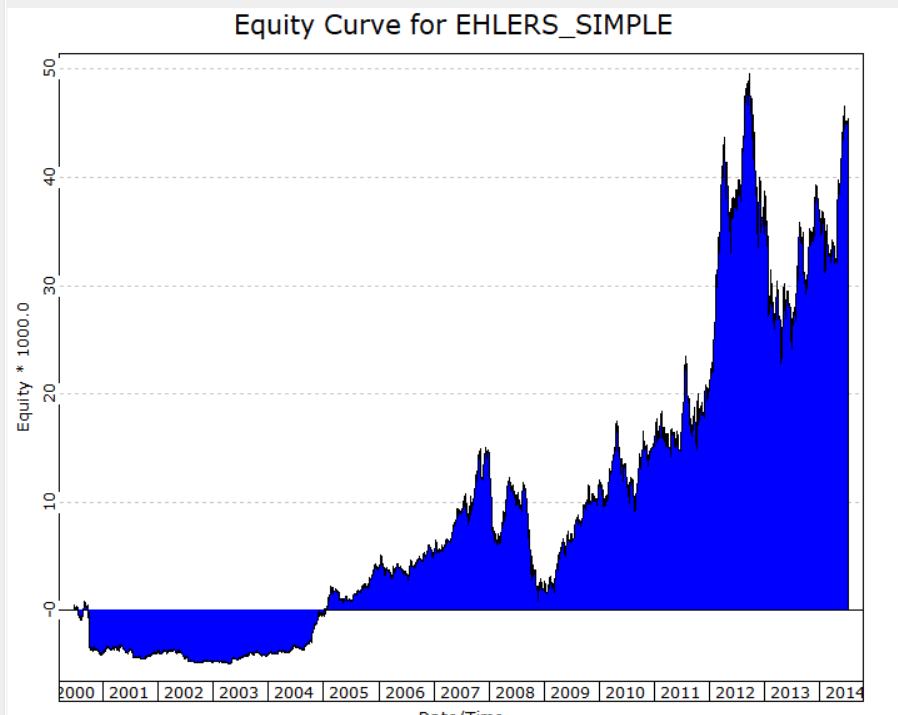
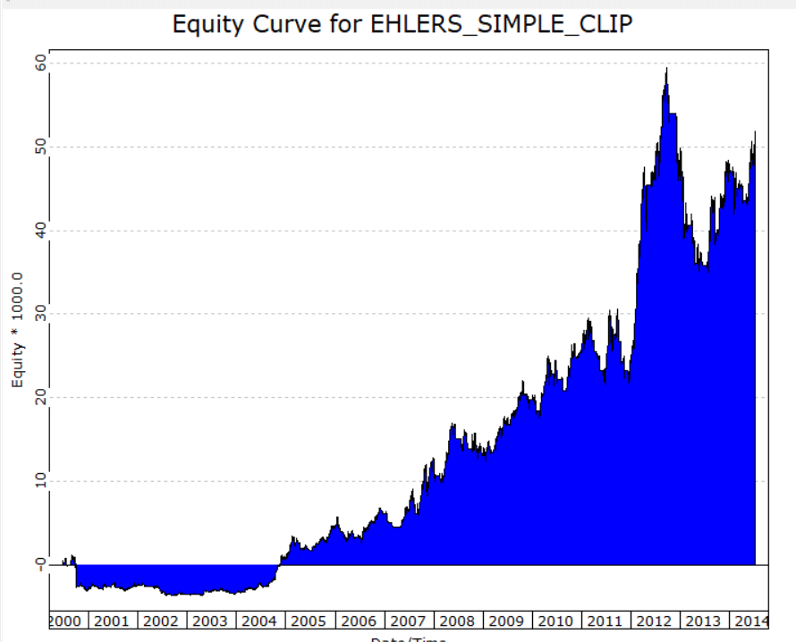
Figure 8 shows the equity curve for the “simple” system trading 100 shares of Apple Inc. (AAPL) from 2000 to 2014. Figure 9 shows the equity curve for the “simple clip” system trading 100 shares of Apple Inc. (AAPL) from 2000 to 2014.

FIGURE 8: TRADERSSTUDIO. Equity curve for the “simple” system trading Apple Inc. (AAPL)

FIGURE 9: TRADERSSTUDIO. Equity curve for the “simple clip” system trading Apple Inc. (AAPL)
—Richard Denning
info@TradersEdgeSystems.com
for TradersStudio
BACK TO LIST

THE ZORRO PROJECT: JUNE 2021
In his article in the May 2021 issue of this magazine (“A Technical Description Of Market Data For Traders”), John Ehlers proposed to treat a price curve like a radio wave, by applying AM and FM demodulating technology. In his article in this issue, “Creating More Robust Trading Strategies With The FM Demodulator,” he describes a practical example of incorporating the FM demodulator into a trading strategy.
The example strategy provided in the article, which was a very simple strategy given only to illustrate how the FM demodulator may be applied and encoded into a strategy, is basically a short-term trend follower. The price curve is differentiated, then integrated again for removing the zero frequency part. The result is smoothed, and the system trades on zero crossings of its rate of change. Two parameters, the smoothing period and the rate-of-change period, are optimized. The code in C for Zorro for replicating this is as follows:
var void simple()
{
  int SigPeriod = optimize(8,6,14,1),
  ROCPeriod = optimize(1,1,6,1);
//Derivative of the price wave
  vars Deriv = series(priceClose(0)-priceClose(2));
//zeros at Nyquist and 2*Nyquist, i.e. Z3 = (1 + Z^-1)*(1 + Z^-2)
  vars Z3 = series(Sum(Deriv,4));
//Smooth Z3 for trading signal
  vars Signal = series(SMA(Z3,SigPeriod));
//Use Rate of Change to identify entry point
  vars Roc = series(Signal[0]-Signal[ROCPeriod]);
//If ROC Crosses Over 0 Then Buy Next Bar on Open;
//If Signal Crosses Under 0 Then Sell Next Bar on Open;
  if(crossOver(Roc,0))
    enterLong();
  else if(crossUnder(Signal,0))
  exitLong();
}
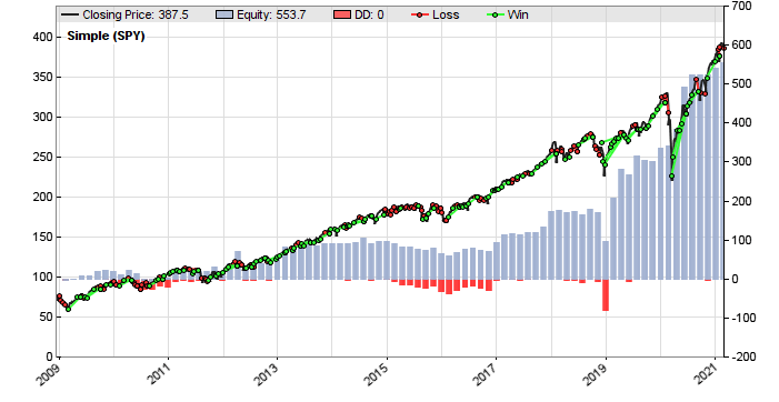
For replicating Ehlers’ results, we use brute force in-sample optimization. This results in an impressive profit factor of almost 3 when applied to the S&P 500 index (SPY) from 2009 to 2021. Still, we can see in the equity curve in Figure 10 that all profit results from the last two years. So, just as Ehlers stated in his article, this is not a very robust system.

FIGURE 10: ZORRO PROJECT. Here is the example simple system without the inclusion of the FM demodulator.
Now we’re going to improve the system by inserting Ehlers’ FM demodulator. The code in C for Zorro to include the FM demodulator is as follows:
void simpleFM()
{
  int i, SigPeriod = optimize(8,6,14,1),
  ROCPeriod = optimize(1,1,6,1);
//Derivative of the price wave
  vars Deriv = series(priceClose(0)-priceClose(2));
//Normalize Degap to half RMS and hard limit at +/- 1
  var RMS = 0;
  for(i=0; i<50; i++) RMS += Deriv[i]*Deriv[i];
  vars Clip = series(clamp(2*Deriv[0]/sqrt(RMS/50),-1,1));
//zeros at Nyquist and 2*Nyquist, i.e. Z3 = (1 + Z^-1)*(1 + Z^-2)
  vars Z3 = series(Sum(Clip,4));
//Smooth Z3 for trading signal
  vars Signal = series(SMA(Z3,SigPeriod));
//Use Rate of Change to identify entry point
  vars Roc = series(Signal[0]-Signal[ROCPeriod]);
//If ROC Crosses Over 0 Then Buy Next Bar on Open;
//If Signal Crosses Under 0 Then Sell Next Bar on Open;
  if(crossOver(Roc,0))
    enterLong();
  else if(crossUnder(Signal,0))
    exitLong();
}
The FM demodulator is basically the clamp() function, which removes the amplitude from the price curve derivative, in combination with the subsequent SMA, which acts as a lowpass filter. The result after brute force optimization is shown in Figure 11.

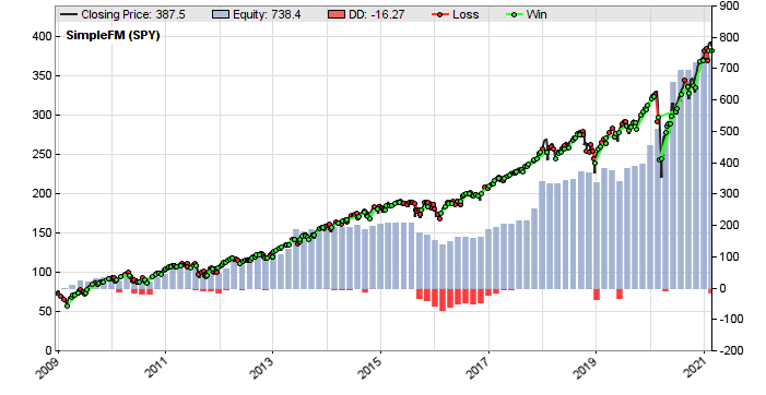
FIGURE 11: ZORRO PROJECT. Here is the example simple system with the inclusion of the FM demodulator.
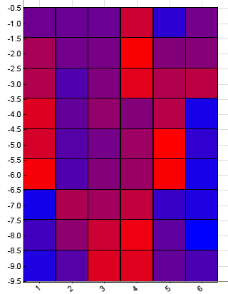
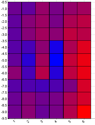
The profit factor is still about the same, slightly below 3, but the equity curve now looks a bit better. Ehlers attributed the increased robustness to the more linear parameter surface. For verifying that, we can export the parameter data from both versions and compare the heatmaps (see Figures 12 & 13).

FIGURE 12: ZORRO PROJECT. This shows a heatmap of the parameters without use of the FM demodulator.

FIGURE 13: ZORRO PROJECT. This shows a heatmap of the parameters with the inclusion of the FM demodulator in the strategy.
The red and blue squares in Figures 12 & 13 are the resulting objectives from the training runs. The more blue, the better the result; red squares indicate bad parameter combinations. We can see that the FM demodulator version has indeed the smoother heatmap with tops in the center. The heatmap of the other system looks crumpled with deep valleys and several tops apart from each other. Clearly, the optimization of the FM demodulator system was more effective.
The code can be downloaded from the 2021 script repository on https://financial-hacker.com. The Zorro platform can be downloaded from https://zorro-project.com.
—Petra Volkova
The Zorro Project by oP group Germany
https://zorro-project.com
BACK TO LIST
MICROSOFT EXCEL: JUNE 2021
In John Ehlers’ article in this issue, “Creating More Robust Trading Strategies With The FM Demodulator,” which is a follow-up to his article last month (“A Technical Description Of Market Data For Traders”), Ehlers walks us through an application of the FM demodulator applied to a relatively simple trading strategy. He provides a three-dimensional modeling of the historical results when applying varying parameters to the basic version of the simple strategy. For comparison, he then applies the same parameter set to a version of the simple strategy that incorporates the FM demodulator.
Be warned—this spreadsheet is quite slow to calculate after any change is made, “time enough to go fetch a coffee” kind of slow! Explanation to follow.
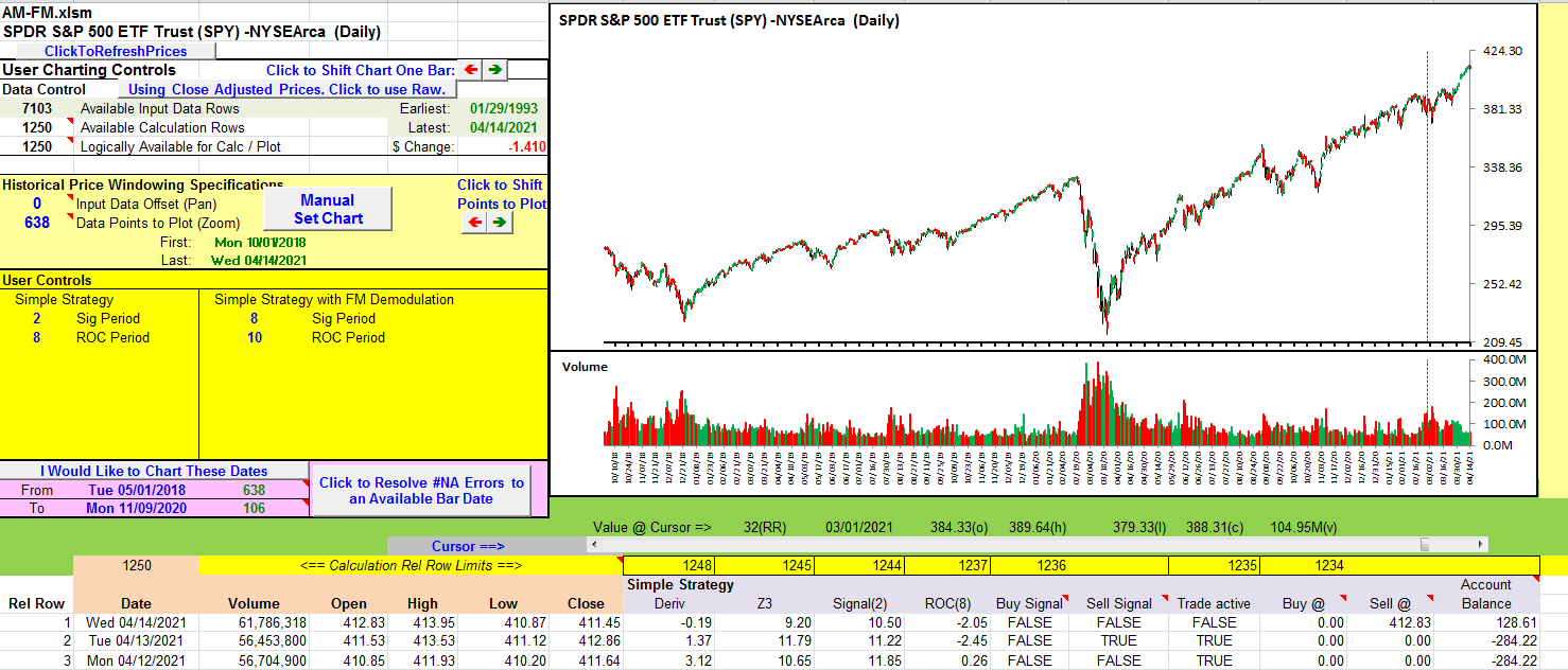
Changing either or both of the user controls for the “simple strategy” will change the “trading” result at the top of the account balance column. This column is a buy and sell running total for the simple strategy. Likewise, changing either or both of the user controls for the “simple strategy with FM demodulator” will change the “trading” result at the top of the account balance column for the “simple strategy with FM demodulator” shown in Figure 14.

FIGURE 14: EXCEL. Basic price and volume chart with user strategy control values showing the computational result at the top of the account balance column.
As is often true with Ehlers’ articles, the basic computations are straightforward and are relatively quick. It is modeling of the scenarios to create the data tables to derive the surface charts that take up the calculation time. This modeling requires one complete computation for each of the possible combinations of sig period and ROC period, then the results of this computation are captured. Rinse and repeat for the next combination of sig period and ROC period. Then do it again for the FM demodulator version. For this spreadsheet, that works out to 36 full computations for the simple strategy and another 36 for the simple strategy with FM.
Enter the data tables feature—an Excel built-in what-if analysis tool. A data table can manage the cycling of up to two distinct parameter sets into their respective control points, calculate the spreadsheet, and then capture the result of each such combination in an X by Y table.
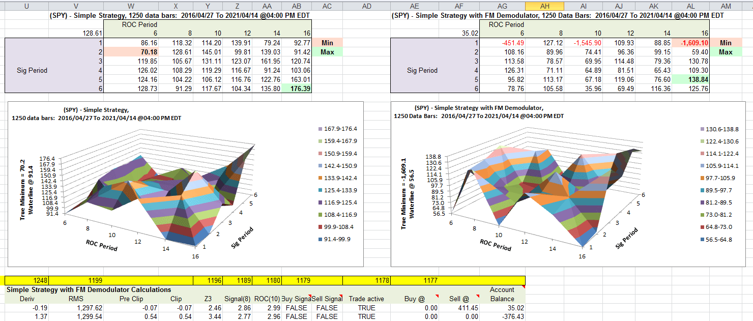
Shown in Figure 15 are two data tables located to the right of the price chart. (Scroll right to view columns U through AM). The data table for the simple strategy occupies cells V3:AB9 and the simple strategy with FM occupies cells AF3:AL9. Evaluating these two data tables consumes computational time.

FIGURE 15: EXCEL. Data tables for the strategies and their corresponding surface charts.
The scenario analysis surface charts appear just below their respective data tables.
Waterlines!
We are primarily interested in finding the best possible parameter combinations. The lowest returns do not contribute much to our search for the best parameter sets and they can take up valuable vertical space on our charts.
In his article, Ehlers uses a “waterline” to ignore the lower, less interesting values, as I have done here. This provides more vertical room to spread the points of more direct interest.
To successfully download a working version of this spreadsheet:
- Right-click on the Excel file link, then
- Select “save as” (or “save target as”) to place a copy of the spreadsheet file on your hard drive.
—Ron McAllister
Excel and VBA programmer
rpmac_xltt@sprynet.com
BACK TO LIST
Originally published in the June 2021 issue of
Technical Analysis of STOCKS & COMMODITIES magazine.
All rights reserved. © Copyright 2021, Technical Analysis, Inc.
