TRADERS’ TIPS
April 2022

For this month’s Traders’ Tips, the focus is Markos Katsanos’ article in this issue, “Stock Market Seasonality.” Here, we present the April 2022 Traders’ Tips code with possible implementations in various software.
You can right-click on any chart to open it in a new tab or window and view it at it’s originally supplied size, often much larger than the version printed in the magazine.
The Traders’ Tips section is provided to help the reader implement a selected technique from an article in this issue or another recent issue. The entries here are contributed by software developers or programmers for software that is capable of customization.

TradeStation: April 2022
Historical data has generally supported the long-standing financial adage “Sell in May and go away, buy in October and stay sober.” Markos Katsanos decided to investigate this apothegm with more recent data, different time periods, and taking into account drawdown and risk-adjusted returns. In his article in this issue, he presents his in-depth findings and possible rational behind them. He then presents his hybrid seasonal system designed to improve on the seasonal systems by adding other technical indicators.
Markos Katsanos’ volume flow indicator (VFI) calculation uses a default period of 130 days for daily charts. As a result, when applying the strategy, you will need to set the maximum number of bars the study will reference in the general tab of properties for all to at least 130. In order to compare the system objectively with the buy & hold results, he specified a trade size as a percent of equity. The supplied strategy code does not have specified trade sizes.
Strategy: TASC APR 2022 Hybrid Seasonal System
// TASC APR 2022
// Seasonal Hybrid System
// Copyright Markos Katsanos 2022

inputs:
	SellMonth( 5 ), // 5 to	8 by 1
	VIXUpMax( 60 ), // 50 to 60 by 10
	Crit( -20 ), 	// -20 to -15 by 5
	K( 1.5 );		// 1.3 to 1.7 by 0.2

variables:
	VIXDown( 0 ),
	VIXUp( 0 ),
	ATRDown( 0 ),
	ATRUp( 0 ),
	RefSymbol( 0, Data2 ),
	VIXClose( 0 ),
	Period( 130 ),
	Coef( 0.2 ),
	VCoef( 2.5 ),
	Cutoff( 0 ),
	MF( 0 ),
	Inter( 0 ),
	VInter( 0 ),
	Vave( 0 ),
	Vmax( 0 ),
	Vc( 0 ),
	VCP( 0 ),
	VFI1( 0 ),
	VFI( 0 ),
	BuySignal( false ),
	VolCondition( false ),
	SellMF( false ),
	SellSeasonal( false ),
	SellVolatility( false );

VIXClose = Close of Data2;

if Highest(VIXClose, 25)[1] <> 0 then
begin
	VIXDown = (VIXClose/Highest(VIXClose, 25)[1]
	 of Data2 - 1) * 100;
end
else
begin
	VIXDown = 0;
end;

if Lowest(VIXClose, 25)[1] <> 0 then
begin
	VIXUp = (VIXClose/Lowest(VIXClose, 25)[1]
	 of Data2 - 1) * 100;
end
else
begin
	VIXUp = 0;
end;

ATRDown = (AvgTrueRange(15)
 /(Highest(AvgTrueRange(15), 25)[1]) - 1) * 100;
ATRUp = (AvgTrueRange(15)
 /(Lowest(AvgTrueRange(15), 25)[1]) - 1) * 100;

Inter = Log( TypicalPrice ) - Log( TypicalPrice[1] );
Vinter = StdDev(inter, 30 );
Cutoff = Coef * Vinter * Close;
Vave = Average( Volume, Period )[1];
Vmax = Vave * Vcoef;
Vc = MinList( Volume, VMax );
MF = TypicalPrice - TypicalPrice[1];

VCP = IFF( MF > Cutoff, VC,
 IFF( MF < -Cutoff, -VC, 0 ) );

VFI1 = Summation( VCP, Period ) / Vave;
VFI = XAverage( VFI1, 3 );

VolCondition = (VIXUp < VIXUpMax or
 ATRUp < K * VIXUpMax) and VFI > Crit;

BuySignal = (Month(Date) >= 10
 or Month(Date) < SellMonth)
 and VolCondition[1];
SellSeasonal = Month(Date)= SellMonth ; // SEASONAL
SellVolatility = VIXUp > 2 * VIXUpMax; // VOLAT EXIT
SellMF = Crit crosses above VFI
 and Average(VFI, 10) < Average(VFI, 10)[1];

if BuySignal then buy this bar at close;

if SellSeasonal then
	Sell ("SELL SEASONAL") this Bar at Close
else if SellVolatility[1] or SellMF[1] then
	Sell ("SELL VOLAT") this Bar at Close;

Indicator: TASC APR 2022 VFI
{
*******************************
VOLUME FLOW INDICATOR (VFI)
Provided By	: MARKOS KATSANOS
Copyright 2004
*******************************
For more information see Markos Katsanos's
articles in the June 2004 and July 2004 issues
of Technical Analysis of Stocks & Commodities
magazine. Period=days for VFI calculation. Default
values are 130 for daily and 26 for weekly charts.
Coef=coefficient for minimal price cut-of (use 0.2
for daily and 0.1 for intraday 5-15 min data)
Vcoef=coefficient for volume cut-off (use 2.5 for
daily and 3.5 for intraday charts)
}

inputs:
	Period( 130 ),
	Coef( .2 ),
	VCoef( 2.5 ),
	SmoothingPeriods( 3 ),
	MA( 30 );

variables:
	TP( 0 ),
	Inter( 0 ),
	VInter( 0 ),
	CutOff( 0 ),
	VAve( 0 ),
	VMax( 0 ),
	VC( 0 ),
	MF( 0 ),
	DirectionalVolume( 0 ),
	myVFI( 0 );

TP = TypicalPrice;

if TP > 0 and TP[1] > 0 then
	Inter = Log(TP) - Log(TP[1])
else
	Inter = 0;

VInter = StdDev( Inter, 30 );
CutOff = Coef * VInter * Close;
VAve = Average(V,Period)[ 1 ];
VMax = VAve * VCoef;
VC = IFF( V < VMax , V, VMax );
MF = TP - TP[1];
DirectionalVolume = IFF( MF > CutOff, +VC,
 IFF( MF < -CutOff, -VC, 0 ) );

if VAve <> 0 then
	myVFI = Summation( DirectionalVolume, Period )
	 / Vave
else
	myVFI = 0;

if SmoothingPeriods > 0 then
	myVFI = XAverage(myVFI, SmoothingPeriods)
else
	myVFI = myVFI;

Plot1( myVFI, "VFI");
Plot2( 0, "0");
Plot3( XAverage(myVFI, MA), "MA" );
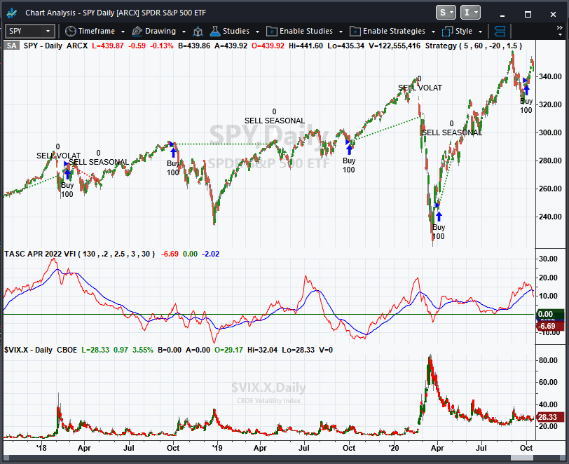
A TradeStation daily chart of the S&P 500 ETF (SPY) and the CBOE Volatility Index ($VIX.X) with the VFI indicator and hybrid seasonal system strategy applied is shown in Figure 1.

FIGURE 1: TRADESTATION. Here is a TradeStation daily chart of the S&P 500 ETF (SPY) and the CBOE Volatility Index ($VIX.X) with the VFI indicator and hybrid seasonal system strategy applied.
This article is for informational purposes. No type of trading or investment recommendation, advice, or strategy is being made, given, or in any manner provided by TradeStation Securities or its affiliates.
—John Robinson
TradeStation Securities, Inc.
www.TradeStation.com
BACK TO LIST

MetaStock: April 2022
In his article “Stock Market Seasonality” in this issue, Markos Katsanos explains a method for trading the market with hybrid seasonal system. His system employs the VFI indicator that Katsanos introduced in 2004. The formulas shown here include the code for the VFI. You must create that indicator first and name it “VFI” and then create the system test.
VFI Indicator:
name: VFI
formula:
VFIPeriod := 130;
Coef:= 0.2;
VCoef:= 2.5;
inter:= Log( Typical() ) - Log( Ref( Typical(), -1 ) );
Vinter:= Stdev(inter, 30 );
Cutoff:= Coef * Vinter * CLOSE;
Vave := Ref( Mov( V, VFIPeriod, S ), -1 );
Vmax := Vave * Vcoef;
Vc := Min( V, Vmax );
MF := Typical() - Ref( Typical(), -1 );
VCP := If( MF > Cutoff, VC, If( MF < -Cutoff, -VC, 0 ) );
VFIa := Sum( VCP , VFIPeriod )/Vave;
If(BarsSince(Cum(1)>268)>=0, Mov( VFIa, 3, E),0);
Seaonal Hybrid System:
Buy Order:
vix:= security("ONLINE:.VIX", C);
VFI:= Fml("VFI");
{Optimizations}
sellmonth:= opt1; {5 - 8, step 1}
vixupmax:= opt2; {50 or 60}
crit:= opt3; {15 or 20}
k:= opt4; {1.3 - 1.7, step 0.2)}
{system calculations}
vixdn:= (vix/ref(hhv(vix,25),-1)-1)*100;
vixup:= (vix/ref(llv(vix,25),-1)-1)*100;
atrdn:= (atr(15)/ref(hhv(atr(15),25),-1)-1)*100;
atrup:= (atr(15)/ref(llv(atr(15),25),-1)-1)*100;
{buy signal}
volcond:= (vixup < vixupmax OR atrup< k*vixupmax) and vfi>crit;
(month() >= 10 or month()<sellmonth) and ref(volcond, -1);

Sell Order:
vix:= security("ONLINE:.VIX", C);
VFI:= Fml("VFI");
{Optimizations}
sellmonth:= opt1; {5 - 8, step 1}
vixupmax:= opt2; {50 or 60}
crit:= opt3; {15 or 20}
k:= opt4; {1.3 - 1.7, step 0.2)}
{system calculations}
vixdn:= (vix/ref(hhv(vix,25),-1)-1)*100;
vixup:= (vix/ref(llv(vix,25),-1)-1)*100;
atrdn:= (atr(15)/ref(hhv(atr(15),25),-1)-1)*100;
atrup:= (atr(15)/ref(llv(atr(15),25),-1)-1)*100;
{sell signal}
sellseason:= Month() = sellmonth;
sellvol:= vixup> 2*vixupmax;
sellmf:= cross(crit, vfi) and mov(vfi,10,s)<Ref(mov(vfi,10,s),-1);
sellseason or ref(sellvol or sellmf, -1);

Optimization Variables:
OPT1:
Description: Sell Month
Minimum: 5
Maximum: 8
Step: 1

OPT2:
Description: Vix Up Max
Minimum: 50
Maximum: 60
Step: 10

OPT3:
Description: VFI Sell
Minimum: 15
Maximum: 20
Step: 5

OPT4:
Description: ATR VIX Ratio
Minimum: 1.3
Maximum: 1.7
Step: 0.2
—William Golson
MetaStock Technical Support
www.MetaStock.com
BACK TO LIST

thinkorswim: April 2022
We put together a strategy based on the article by Markos Katsanos in this issue, “Stock Market Seasonality.” We built this using our proprietary scripting language, thinkscript. To ease the loading process, simply open the link https://tos.mx/acCJizc or enter the address into setup→open shared item from within thinkorswim and choose view thinkscript strategy and name it “HybridSeasonalStrategy” or something you can easily remember. You will then be able to add the strategy to your charts under the edit studies menu and selecting the strategies subtab.
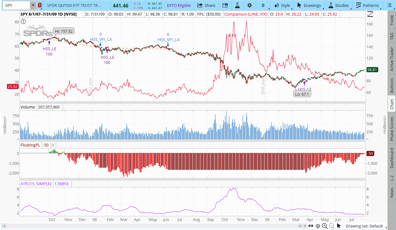
The strategy can be seen on a chart of SPY for August 2007 through July 2009 along with the ATR and VIX comparison studies in Figure 2. Please see Markos Katsanos’ article in this issue for more information on how to read the chart and utilize the strategy.

FIGURE 2: THINKORSWIM. The strategy can be seen on a chart of SPY for August 2007 through July 2009 along with the ATR and VIX comparison studies.
—thinkorswim
A division of TD Ameritrade, Inc.
www.thinkorswim.com
BACK TO LIST

eSIGNAL: April 2022
For this month’s Traders’ Tip, we’ve provided the study “Elegant Oscillator.efs” based on the article by John Ehlers in the February 2022 issue, “Inverse Fisher Transform Redux.”
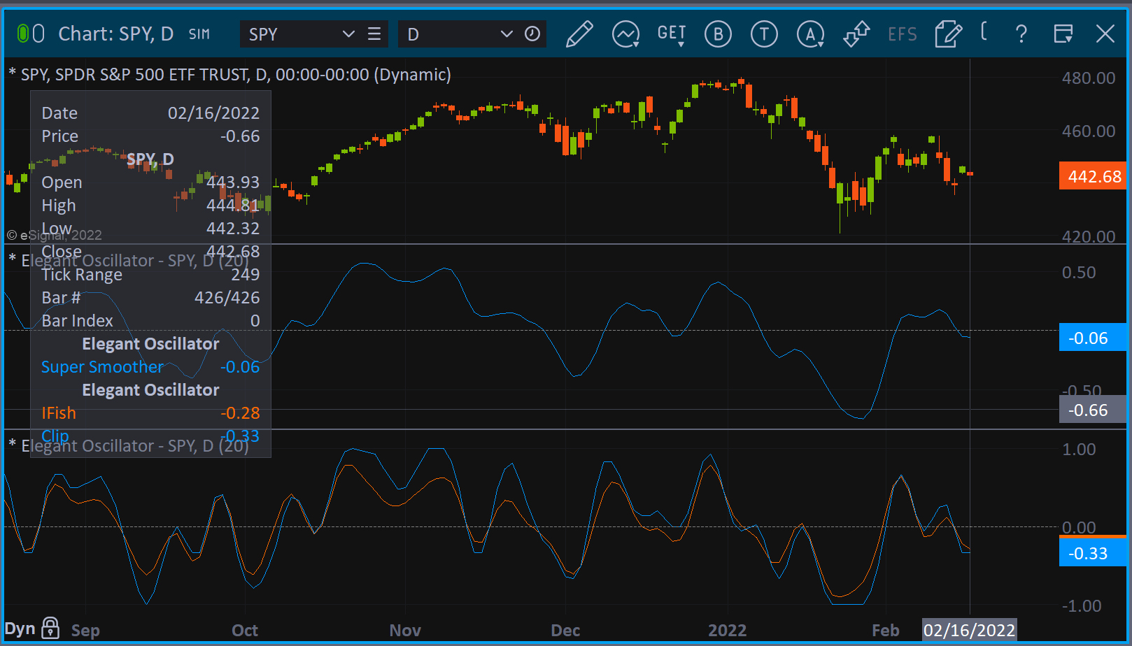
The study contains formula parameters that may be configured through the edit chart window (right-click on the chart and select “edit chart”). A sample chart is shown in Figure 3.

FIGURE 3: eSIGNAL. Here is an example of the study plotted on a daily chart of $SPX.
To discuss this study or download a complete copy of the formula code, please visit the EFS library discussion board forum under the forums link from the support menu at www.esignal.com or visit our EFS KnowledgeBase at https://www.esignal.com/support/kb/efs. The eSignal formula script (EFS) is also available for copying & pasting here:
/**********************************
Provided By:
Copyright 2019 Intercontinental Exchange, Inc. All Rights Reserved.
eSignal is a service mark and/or a registered service mark of Intercontinental Exchange, Inc.
in the United States and/or other countries. This sample eSignal Formula Script (EFS)
is for educational purposes only.
Intercontinental Exchange, Inc. reserves the right to modify and overwrite this EFS file with each new release.

Description:
    Inverse Fisher Transform Redux
    by John F. Ehlers


Version:            1.00  11/02/2022

Formula Parameters:                    Default:
BandEdge                               20


Notes:
The related article is copyrighted material. If you are not a subscriber
of Stocks & Commodities, please visit www.traders.com.

**********************************/
var fpArray = new Array();
var bInit = false;

function preMain() {
    setStudyTitle("Elegant Oscillator");
    setCursorLabelName("Super Smoother", 0);
    setCursorLabelName("IFish", 1);
    setCursorLabelName("Clip", 2);
    setPriceStudy(false);
    setDefaultBarFgColor(Color.RGB(0x00,0x94,0xFF), 0);
    setDefaultBarFgColor(Color.RGB(0xFE,0x69,0x00), 1);
    setDefaultBarFgColor(Color.RGB(0x00,0x94,0xFF), 2);
    setPlotType( PLOTTYPE_LINE , 0 );


    var x=0;
    fpArray[x] = new FunctionParameter("BandEdge", FunctionParameter.NUMBER);
	with(fpArray[x++]){
        setLowerLimit(1);
        setDefault(20);
    }
}

var bVersion = null;
var xClose = null;
var xDeriv = null;
var xRMS = null;
var xNDeriv = null;
var xIFish = null;
var SS = null;
var SS_1 = null;
var SS_2 = null;
var a1 = null;
var b1 = null;
var c1 = null;
var c2 = null;
var c3 = null;
var xInteg = null;
var xClip = null;
var xIntegClip = null;

function main(BandEdge) {
    if (bVersion == null) bVersion = verify();
    if (bVersion == false) return;

    if ( bInit == false ) {
        xClose = close();
        addBand(0, PS_DASH, 1, Color.grey, 1);
        xDeriv = efsInternal('Calc_Deriv', xClose);
        xNDeriv = efsInternal('Calc_NDeriv', xDeriv);
        xIFish = efsInternal('Calc_IFish', xNDeriv);
        SS = null;
        SS_1 = null;
        SS_2 = null;
        a1 = Math.pow(Math.E, -Math.SQRT2 * Math.PI / BandEdge);
        b1 = 2 * a1 * Math.cos(Math.SQRT2 * Math.PI / BandEdge);
        c2 = b1;
        c3 = -a1 * a1;
        c1 = 1- c2 - c3;
        xInteg = efsInternal('Calc_Integ', xIFish);
        xClip = efsInternal('Calc_Clip', xDeriv);
        xIntegClip = efsInternal('Calc_Integ', xClip);

        bInit = true;
    }

    if (getCurrentBarCount() < 50) return;
    if (getBarState() == BARSTATE_NEWBAR) {
        SS_2 = SS_1;
        SS_1 = SS;
        SS = 0;
    }
    SS = c1 * (xIFish.getValue(0) + xIFish.getValue(-1)) / 2 + c2 * SS_1 + c3 * SS_2;

    return [SS, xInteg.getValue(0), xIntegClip.getValue(0)];
}

function Calc_Clip(xDeriv){
    ret = xDeriv.getValue(0);

    if (ret > 1) ret = 1;
    if (ret < -1) ret = -1;

    return ret;
}

function Calc_Integ(xSeries){
    ret = 0;
    ret = xSeries.getValue(0) + 2 * xSeries.getValue(-1) + 3 * xSeries.getValue(-2) + 3 * xSeries.getValue(-3) + 2 * xSeries.getValue(-4) + xSeries.getValue(-5);
    return (ret / 12);
}

function Calc_IFish(xNDeriv){
    ret = 0;
    ret = (Math.pow(Math.E, 2 * xNDeriv.getValue(0)) - 1) / (Math.pow(Math.E, 2 * xNDeriv.getValue(0)) + 1)

    return ret;
}

function Calc_NDeriv(xDeriv){
    ret = 0;
    RMS  = 0;
    for (var i = 0; i < 50; i++) {
        RMS = RMS + xDeriv.getValue(-i) * xDeriv.getValue(-i);
    }
    if (RMS != 0) {
        RMS = Math.sqrt(RMS / 50);
        ret = xDeriv.getValue(0) / RMS;
    }
    return ret;
}

function Calc_Deriv(xClose){
    ret = 0;
    ret = xClose.getValue(0) - xClose.getValue(-2);
    return ret;
}

function verify(){
    var b = false;
    if (getBuildNumber() < 779){

        drawTextAbsolute(5, 35, "This study requires version 10.6 or later.",
            Color.white, Color.blue, Text.RELATIVETOBOTTOM|Text.RELATIVETOLEFT|Text.BOLD|Text.LEFT,
            null, 13, "error");
        drawTextAbsolute(5, 20, "Click HERE to upgrade.@URL=https://www.esignal.com/download/default.asp",
            Color.white, Color.blue, Text.RELATIVETOBOTTOM|Text.RELATIVETOLEFT|Text.BOLD|Text.LEFT,
            null, 13, "upgrade");
        return b;
    }
    else
        b = true;

    return b;
}
—Eric Lippert
eSignal, an Interactive Data company
800 779-6555, www.eSignal.com
BACK TO LIST

Wealth-Lab.com: April 2022
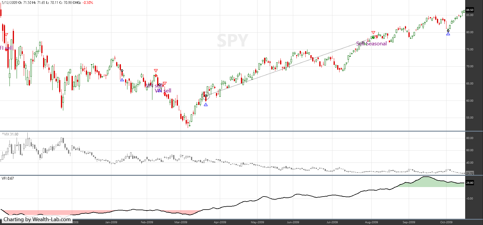
We have coded the seasonal hybrid system presented in Markos Katsanos’ article in this issue for the benefit of Wealth-Lab 7 users.
To get the ^VIX data for backtesting, make sure to check “Yahoo! Finance” or other supported data source in the Data Manager (historical providers tab). As icing on the cake, in Figure 4, its history is plotted as candlesticks rather than as a line chart.

FIGURE 4: WEALTH-LAB. This shows sample trades taken by the system applied to a daily chart of SPY.
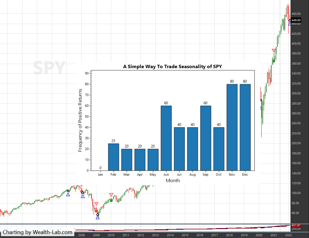
On a related note, we wanted to remind motivated traders about a different way to gauge the monthly seasonality. A trading system for Wealth-Lab 7 based on the frequency of positive monthly returns introduced by Perry Kaufman was featured in the September 2019 issue in the Traders’ Tips section (see Figure 5). Its code is available here:
https://www.wealth-lab.com/Discussion/Traders-39-Tips-2019-09-A-Simple-Way-to-Trade-Seasonality-Kaufman-7566

FIGURE 5: WEALTH-LAB. A plot with a distribution of monthly returns reveals that the second half of the year’s months have been benevolent for trading in SPY in the last two decades.
using WealthLab.Backtest;
using System;
using WealthLab.Core;
using WealthLab.Indicators;
using System.Drawing;
using System.Collections.Generic;
using WealthLab.TASC;

namespace WealthScript1
{
public class SeasonalHybridSystem : UserStrategyBase
{

public SeasonalHybridSystem() : base()
{
AddParameter("Sell month", ParameterTypes.Int32, 8, 5, 8, 1);
AddParameter("VIX up max", ParameterTypes.Int32, 60, 50, 60, 10);
AddParameter("VFI sell", ParameterTypes.Int32, -20, -20, -15, 5); /* VFI sell */
AddParameter("ATR/VIX Ratio", ParameterTypes.Double, 1.5, 1.3, 1.7, 0.2);
}

/* create indicators and other objects here, this is executed prior to the main trading loop */

public override void Initialize(BarHistory bars)
{
sellMonth = Parameters[0].AsInt;
vixUpMax = Parameters[1].AsInt;
vfiSell = Parameters[2].AsInt;
atrVixRatio = Parameters[3].AsDouble;

/* obtain the VIX from Yahoo */

vix = GetHistory( bars, "^VIX");
vixDn = ((vix.Close
/ Highest.Series(vix.Close,25)>>1) - 1) * 100;

            vixUp = ((vix.Close
/ Lowest.Series(vix.Close,25)>>1) - 1) * 100;
atr = ATR.Series(bars, 15);
atrDn = ((atr
/ Highest.Series(atr, 25) >> 1) - 1) * 100;

            atrUp = ((atr
/ Lowest.Series(atr, 25) >> 1) - 1) * 100;

vfi = VFI.Series(bars, 130, 3, 0.2, 2.5);
PlotBarHistoryStyle( vix, "vix", "VIX");
PlotTimeSeriesOscillator( vfi, "VFI", "vfi", -20, +20, default, Color.Red, Color.Green);
StartIndex = 130;
}

/* execute the strategy rules here, this is executed once for each bar in the backtest history */

public override void Execute(BarHistory bars, int idx)
{
/* Buy conditions */

bool volCondition = (vixUp[idx] < vixUpMax) || (atrUp[idx] < atrVixRatio * vixUpMax) && vfi[idx] > vfiSell;
bool volConditionRef = (vixUp[idx-1] < vixUpMax || atrUp[idx-1] < atrVixRatio * vixUpMax) && vfi[idx-1] > vfiSell;
bool buy = (bars.DateTimes[idx].Month >= 10 ||  bars.DateTimes[idx].Month < sellMonth) && volConditionRef;
bool sellSeasonal = bars.DateTimes[idx].Month == sellMonth;
bool sellVolatility = vixUp[idx] > 2 * vixUpMax;
bool sellVolatilityRef = vixUp[idx-1] > 2 * vixUpMax;
bool sellMF = vfi.CrossesUnder(vfiSell,idx) && SMA.Series(vfi,10)[idx] < SMA.Series(vfi,10)[idx-1];
bool sellMFRef = vfi.CrossesUnder(vfiSell,idx-1) && SMA.Series(vfi,10)[idx-1] < SMA.Series(vfi,10)[idx-2];
bool sell = sellSeasonal || sellVolatilityRef || sellMFRef;

if (!HasOpenPosition(bars, PositionType.Long))
{
/* code your buy conditions here */
if (buy)
PlaceTrade( bars, TransactionType.Buy, OrderType.Market);
}

else

{
/* code your sell conditions here */

if (sell)
{
string sellSignal = sellSeasonal ? "Sell Seasonal" : sellVolatilityRef ? "High volatility sell" : "VFI sell";
DrawBarAnnotation( sellSignal, idx, false, Color.Purple, 18, true);
ClosePosition( LastPosition, OrderType.Market, default, sellSignal);
}
}
}

/* declare private variables below */

BarHistory vix;
TimeSeries atr, vixDn, vixUp, atrDn, atrUp, vfi;
int sellMonth = 8, vixUpMax = 60, vfiSell = -20;
double atrVixRatio = 1.5;
}
}
—Gene Geren (Eugene)
Wealth-Lab team
www.wealth-lab.com
BACK TO LIST

NinjaTrader: April 2022
The “S&P 500 Seasonal System Strategy” as described by Markos Katsanos in his article in this issue, “Stock Market Seasonality,” is available for download at the following links for NinjaTrader 8 and NinjaTrader 7:
Once the file is downloaded, you can import the strategy into NinjaTrader 8 from within the control center by selecting Tools→Import→NinjaScript Add-On and then selecting the downloaded file for NinjaTrader 8. To import in NinjaTrader 7 from within the control center window, select the menu File→Utilities→Import NinjaScript and select the downloaded file.
You can review the strategy source code in NinjaTrader 8 by selecting the menu New→NinjaScript Editor→Strategies folder from within the Control Center window and selecting the SP500SeasonalSystem file. You can review the strategy source code in NinjaTrader 7 by selecting the menu Tools→Edit NinjaScript→Strategy from within the control center window and selecting the SP500SeasonalSystem file.
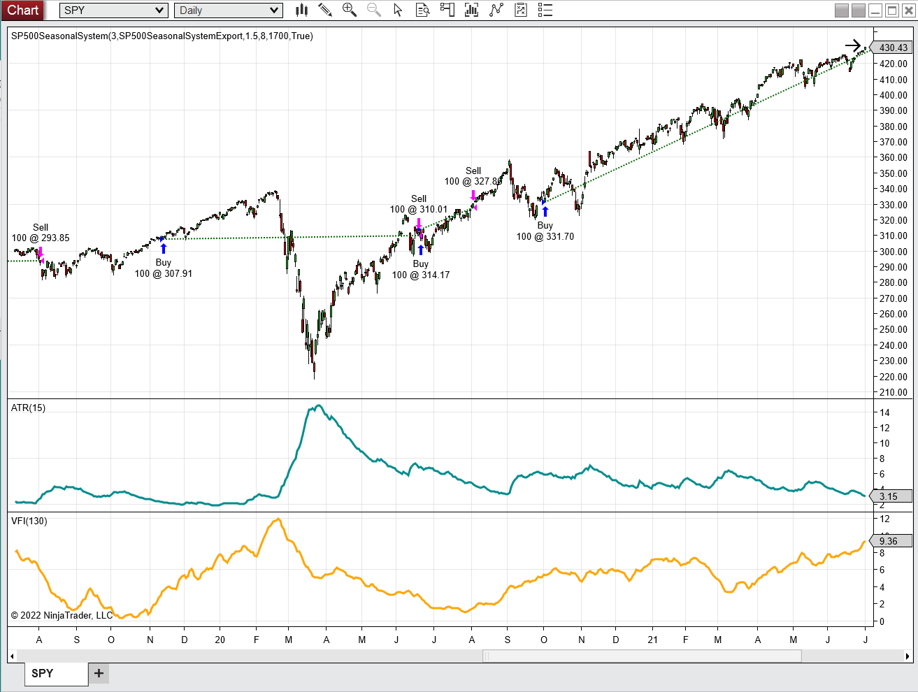
A sample chart displaying the strategy is shown in Figure 6.

FIGURE 6: NINJATRADER. The SP500SeasonalSystem strategy displayed on a SPY chart from July 2019 to July 2021. Note: Volume-related parameters are modified to better fit volume read from a Kinetick datafeed.
NinjaScript uses compiled DLLs that run native, not interpreted, to provide you with the highest performance possible.
—Chris Lauber
NinjaTrader, LLC
www.ninjatrader.com
BACK TO LIST

Neuroshell Trader: April 2022
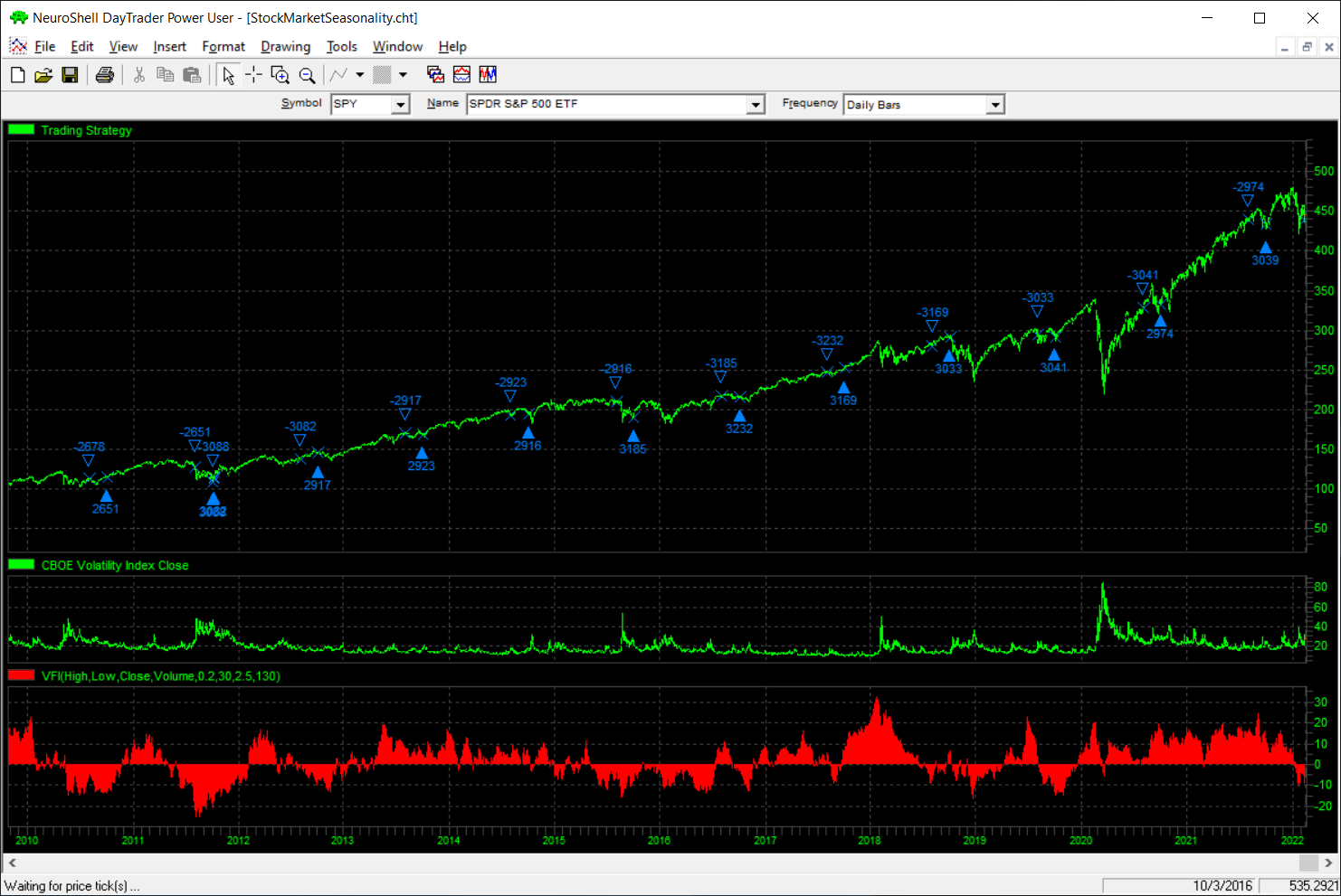
The hybrid seasonal system presented in Markos Katsanos’ article in this issue can be easily implemented in NeuroShell Trader by combining a few of NeuroShell Trader’s 800+ indicators in a trading system. To implement the hybrid seasonal system, select new strategy from the insert menu and use the trading strategy wizard to create the following strategy:
BUY LONG CONDITIONS: [All of which must be true]
     Or2(A>=B(Month of Year(Date),10),A<B(Month of Year(Date),8))
     Or2(A<B(Divide(CBOE Volatility Index Close,Lag(Min(CBOE Volatility Index Close,25),1)),1.6),  A<B(Divide(ATR(High,Low,Close,15),Lag(Min(ATR(High,Low,Close,15),25),1)),1.9))
     A>B(VFI(High,Low,Close,Volume,0.2,30,2.5,130),-20)

SELL LONG CONDITIONS: [1 of which must be true]
     August Flag(Date)
     A>B(Divide(CBOE Volatility Index Close,Lag(Max(CBOE Volatility Index Close,25),1)),2.2)
     And2(CrossBelow(VFI(High,Low,Close,Volume,0.2,30,2.5,130),-20), A<B(Momentum(Avg(VFI(High,Low,Close,Volume,0.2,30,2.5,130),10),1),0))
Note that this system uses the volume flow custom indicator, which can be created by selecting new indicator from the insert menu and using the indicator wizard to create the following indicators:
TYPICAL:  	Avg3 ( High, Low, Close)
CUTOFF:  	Multiply3 ( 0.2, StndDev ( Momentum (Ln (TYPICAL),1), 30 ), Close )
VAVE:  	LagAvg ( Volume, 1, 130 )
VC:  	Min2 ( Volume, Multiply2 ( 2.5, VAVE ) )
MF :  	Momentum (TYPICAL, 1 )

VFI:  	Divide ( Sum( IfThenIfThenElse ( A>B(MF,CUTOFF), VC,
A<B(MF, Negative(CUTOFF)), Negative(VC), 0 ), 130 ), VAVE )
Users of NeuroShell Trader can go to the Stocks & Commodities section of the NeuroShell Trader free technical support website to download a sample chart which includes the volume flow indicator.

FIGURE 7: NEUROSHELL TRADER. This NeuroShell Trader chart displays a chart of the NeuroShell hybrid seasonal system.
—Ward Systems Group, Inc.
sales@wardsystems.com
www.neuroshell.com
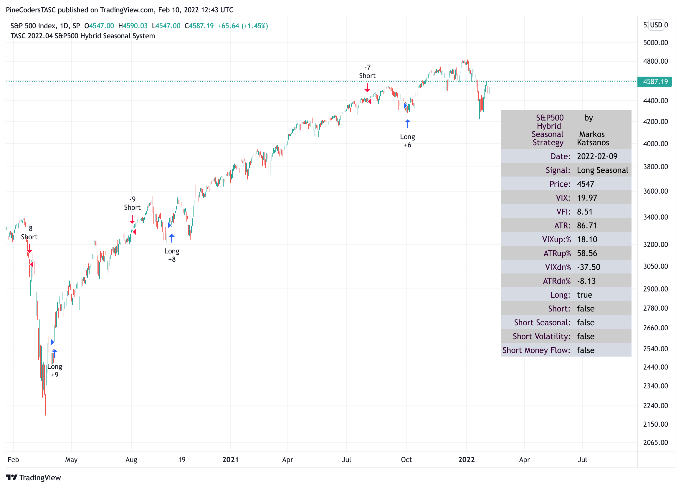
BACK TO LIST

TradingView: April 2022
Here is the TradingView Pine Script code for implementing the hybrid seasonal system described in this issue’s article by Markos Katsanos, “Stock Market Seasonality.”
//  TASC Issue: April 2022 - Vol. 40, Issue 5
//  Article: Sell In May? Stock Market Seasonality
//  Article By: Markos Katsanos
//    Language: TradingView's Pine Script v5
// Provided By: PineCoders, for tradingview.com

//@version=5
strategy("TASC 2022.04 S&P500 Hybrid Seasonal System",
 default_qty_type=strategy.percent_of_equity,
 commission_type=strategy.commission.percent,
 currency=currency.USD,
 overlay=true,
 initial_capital=100000,
 commission_value=0.01,
 default_qty_value=10)

volatility (float Src, int Period) =>
    [(Src / ta.highest(Src, Period)[1] - 1.0) * 100.0,
     (Src / ta.lowest (Src, Period)[1] - 1.0) * 100.0]

// ref: https://mkatsanos.com/volume-flow-vfi-indicator/
vfi(int Period=130, float VCoef=2.5, float Coef=0.2) =>
    lastHLC3 = nz(hlc3[1], hlc3)
    MF     = hlc3 - lastHLC3
    Vinter = ta.stdev(math.log(hlc3) - math.log(lastHLC3), 30)
    Vave   = ta.sma(volume, Period)[1]
    Cutoff = Coef * close * Vinter
    VC     = math.min(volume, Vave * VCoef)
    VCP    = MF >  Cutoff ?  VC :
             MF < -Cutoff ? -VC : 0.0
    VFI1   = math.sum(VCP, Period) / Vave
    VFI    = ta.ema(VFI1, 3)

ig_so = "Short Signal Options"
i_sMonth = input.int(8, "Sell Month:",  1, 12, 1, group=ig_so,
                  tooltip="The worst performing month.")
i_maxVI = input.int(60, "Max VIX up:", 50, 60, 5, group=ig_so,
                  tooltip="maximum VIX volatility threshold")
i_critVFI = input.int(-20, "Critical VFI Sell:", -20, -15, 5,
     group=ig_so, tooltip="Critical VFI threshold")
i_K = input.float(1.5, "ATR/VIX Ratio:", 1.3, 1.7, 0.2,
     group=ig_so, tooltip="ATR to VIX ratio for sell signal")

i_showT = input.bool(true, " - Display Table")
i_Tpos  = input.string(position.middle_right, "Position:",
 options=[position.top_left,      position.middle_left,
          position.bottom_left,   position.top_center,
          position.middle_center, position.bottom_center,
          position.top_right,     position.middle_right,
          position.bottom_right])

// Comparison Index
VIX = request.security("VIX", timeframe.period, close)
[VIXdn, VIXup] = volatility(       VIX, 25) // Implied
[ATRdn, ATRup] = volatility(ta.atr(15), 25) // Historical
VFI   = vfi()
VFI10 = ta.sma(VFI, 10)

lowVolat  = VIXup < i_maxVI or ATRup < (i_K * i_maxVI)
VolatCnd  = VFI > i_critVFI ? lowVolat : false
BUY       = (month <  i_sMonth or month >= 10) and VolatCnd[1]
SEASONAL  =  month == i_sMonth      //   SEASONAL EXIT
VOLATIL   = (VIXup > (2 * i_maxVI)) // VOLATILITY EXIT
MNYFLOW   = ta.cross(i_critVFI, VFI) and VFI10 < VFI10[1]
SELL      = SEASONAL or VOLATIL[1] or MNYFLOW[1]

LONG  = strategy.long
SHORT = strategy.short
if strategy.equity > 0
    strategy.entry("Long",              LONG, when=BUY)
    strategy.entry("Short",            SHORT, when=SELL)
    strategy.entry("Short Seasonal",   SHORT, when=SEASONAL)
    strategy.entry("Short Volatility", SHORT, when=VOLATIL[1])
    strategy.entry("Short MF Crit.",   SHORT, when=MNYFLOW[1])

atr10 = ta.atr(10)
date  = str.format("{0,number,0000}-{1,number,00}" +
       "-{2,number,00}", year, month, dayofmonth)
SIGNAL = switch
    BUY                 => "Long Seasonal"
    SELL and SEASONAL   => "Short Seasonal"
    SELL and VOLATIL[1] => "Short Volatility"
    SELL and MNYFLOW[1] => "Short MF Bearish"
    => "Exit"

var string[] leftLabels = array.from(
 "S&P500   \nHybrid    \nSeasonal   \nStrategy   ", "Date:",
 "Signal:", "Price:", "VIX:", "VFI:", "ATR:", "VIXup:%",
 "ATRup%", "VIXdn%", "ATRdn%", "Long:", "Short:",
 "Short Seasonal:", "Short Volatility:", "Short Money Flow:")
evn = #D6DAE3, color odd = #CCCCCC
var dTable = table.new(i_Tpos, 2, 17, #00000080)
if i_showT and barstate.islastconfirmedhistory
    string[] rightLabels = array.from(
     "   by\n\n Markos\nKatsanos",str.tostring(date),
     str.tostring(SIGNAL),        str.tostring(open),
     str.tostring(VIX),           str.tostring( VFI,   ".00"),
     str.tostring(atr10, ".00"),  str.tostring(VIXup,  ".00"),
     str.tostring( ATRup, ".00"), str.tostring(VIXdn,  ".00"),
     str.tostring( ATRdn, ".00"), str.tostring(BUY),
     str.tostring(   SELL),       str.tostring(SEASONAL),
     str.tostring(VOLATIL),       str.tostring(MNYFLOW))
    for _i=0 to 15
        table.cell(dTable, 0, _i, array.get( leftLabels, _i),
         0,0, #330033, text.align_right, bgcolor=_i%2?evn:odd)
        table.cell(dTable, 1, _i, array.get(rightLabels, _i),
         0,0, #000000, text.align_left,  bgcolor=_i%2?evn:odd)

FIGURE 8: TRADINGVIEW. Shown here is an example of the seasonal hybrid system.
The indicator is available on TradingView from the PineCodersTASC account:
www.tradingview.com/u/PineCodersTASC/#published-scripts
—PineCoders, for TradingView
www.TradingView.com
BACK TO LIST

AIQ: April 2022
The importable AIQ EDS file based on Markos Katsanos’ article in this issue, “Stock Market Seasonality,” can be obtained on request via email to info@TradersEdgeSystems.com. The code is also available below.
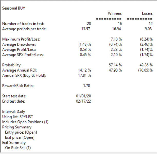
Code for the author’s system is set up in the AIQ code file. Figure 9 shows a summary EDS backtest of the system using the SPY ETF from 1/1/2000 to 2/17/2022.

FIGURE 9: AIQ. This shows the summary EDS backtest of the system using the SPY ETF from 1/1/2000 to 2/17/2022.
!Stock Market Seasonality
!Author: Markos Katsanos, TASC April 2022
!Coded by: Richard Denning, 2/10/2022

C is [close].
C1 is valresult(C,1).
H is [high].
L is [low].
V is [volume].
Avg is (H+L+C)/3.

VIXc is TickerUDF("VIX",C).
VIXc1 is valresult(VIXc,1).
VIXllv is lowresult(VIXc,25).
VIXllv1 is valresult(VIXllv,1).
VIXhhv is highresult(VIXc,25).
VIXhhv1 is valresult(VIXhhv,1).
VIXDN is (VIXc1 / VIXhhv1)*100.
VIXUP is (VIXc1 / VIXllv1)*100.

TR is max(max(C1-L,H-C1),H-L).
ATR is expavg(TR,15*2-1).
ATR1 is valresult(ATR,1).
ATRllv is highresult(ATR,25).
ATRllv1 is valresult(ATRllv,1).
ATRhhv is highresult(ATR,25).
ATRhhv1 is valresult(ATRhhv,1).
ATRDN is (ATR1 / ATRhhv1)*100.
ATRUP is  (ATR1 / ATRllv1)*100.

!VFI
Period is 130.
Coef is 0.2.
VCoef is 2.5.

inter is ln( Avg ) - ln( valresult( Avg, 1) ).
Vinter is Sqrt(variance(inter, 30 )).
Cutoff is Coef * Vinter * C.
Vave is valresult( simpleavg( V, Period ), 1 ).
Vmax is Vave * Vcoef.
VC is Min( V, Vmax ).
MF is Avg - valresult( Avg, 1 ).
VCP is iff(MF > Cutoff, VC, iff(MF < -Cutoff, -VC, 0 )).
VFI1 is Sum( VCP, Period ) / Vave.
VFI is expavg( VFI1, 3 ).

SELLMONTH is 8.
VIXUPMAX is 60.
CRIT is -20. !VFI SELL
K is 1.5.  !ATR/VIX RATIO
VOLCONDITION is (VIXUP<VIXUPMAX OR ATRUP<K*VIXUPMAX ) AND VFI>CRIT.
BUY if (Month()>=10 OR Month()<SELLMONTH) AND valresult(VOLCONDITION,1).
SELLSEASONAL if Month() = SELLMONTH. !SEASONAL
SELLVOLATILITY if VIXUP>2*VIXUPMAX. !VOLATILITY EXIT
SELLMF if CRIT > VFI AND valrule(CRIT < VFI,1) AND simpleavg(VFI,10)<valresult(simpleavg(VFI,10),1).
Sell if SELLSEASONAL OR valrule(SELLVOLATILITY,1) OR valrule(SELLMF,1).
—Richard Denning
info@TradersEdgeSystems.com
for AIQ Systems
BACK TO LIST

The Zorro Project: April 2022
In his article in this issue, Markos Katsanos examines the saying to “sell in May and go away.” Following is the C code translation for the AmiBroker code given in his article’s sidebar, except that we’ve moved his VFI (volume flow indicator) code to a separate indicator function to avoid having the trading logic cluttered with indicator code. Here is the C code for use in Zorro:
asset("SPY");
if(month() == 8 && tdm() == 1) // sell 1st trading day of August,
	exitLong();
else if(month() == 10 && tdm() == 1) // buy back 1st trading day of October
	enterLong();
var priceAvg(int Offset) {
	return (priceC(Offset)+priceH(Offset)+priceL(Offset))/3;
}

var VFI(var Period,var Coef, var VCoef)
{
	vars Inters = series(log(priceAvg(0))-log(priceAvg(1)));
	var Vinter = StdDev(Inters,30);
	var Cutoff = Coef * Vinter * priceC();
	vars Volumes = series(marketVol());
	var Vave = SMA(Volumes+1,Period);
	var Vmax = Vave * VCoef;
	var VC = min(Volumes[0],Vmax);
	var MF = priceAvg(0)-priceAvg(1);
	vars VCPs = series(ifelse(MF > Cutoff,VC,ifelse(MF < -Cutoff,-VC,0)));
	var VFI1 = Sum(VCPs,Period)/Vave;
	return EMA(VFI1,3);
}

function run()
{
	StartDate = 2006;
	EndDate = 2022;
	BarPeriod = 1440; // 1 day
	LookBack = 150;

	assetList("AssetsIB");
	MaxLong = 1;
	Capital = 100000;
	Margin = Equity; // invest all you have
	Leverage = 1;
	BarZone = EST;
	Fill = 3; // enter/exit at next day open
	set(PARAMETERS,TESTNOW,PLOTNOW);

	asset("VIX");
	var VIXdn = (priceC(0)/HH(25,0)-1)*100;
	var VIXup = (priceC(0)/LL(25,0)-1)*100;

	asset("SPY");
	int SellMonth = optimize(8,5,8,1);
	var VIXupMax = optimize(60,50,60,10);
	var Crit = -optimize(20,15,20,5); //VFI SELL
	var K = optimize(1.5,1.3,1.7,.2); // ATR/VIX RATIO

	vars ATRs = series(ATR(15));
	var ATRDn = (ATRs[0]/MaxVal(ATRs,25)-1)*100;
	var ATRUp = (ATRs[0]/MinVal(ATRs,25)-1)*100;

	vars VFIs = series(VFI(130,0.2,2.5));
	vars SMAVFIs = series(SMA(VFIs,10));
	bool VolCondition = (VIXup < VIXupMax || ATRUp < K*VIXupMax ) && VFIs[0] > Crit;
	bool Buy = (month() >= 10 || month() < SellMonth) && ref(VolCondition,1) != 0;
	bool SellSeasonal = month() == SellMonth ; //SEASONAL
	bool SellVolatility = VIXup > 2*VIXupMax ; //VOLATILITY EXIT
	bool SellMF = crossUnder(VFIs,Crit) && SMAVFIs[0] < SMAVFIs[1] ;
	bool Sell = SellSeasonal || ref(SellVolatility,1) != 0 || ref(SellMF,1) != 0;

	if(Sell)
		exitLong();
	else if(Buy)
		enterLong();
}
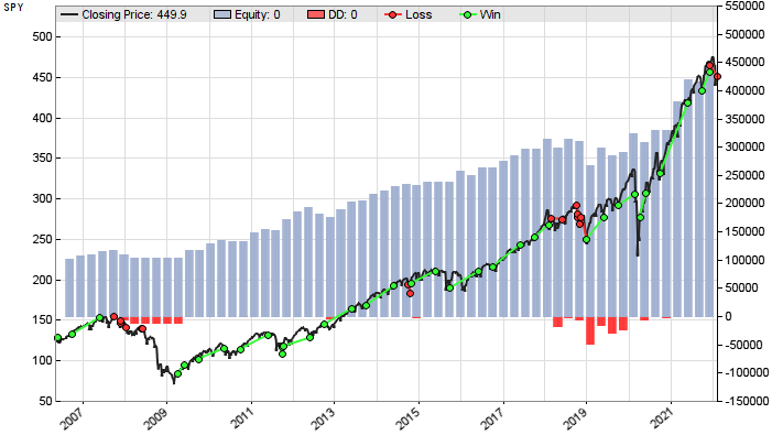
A chart in Zorro can be seen in Figure 10.

FIGURE 10: ZORRO PROJECT. Here is the author’s seasonal system shown on a sample chart.
The VFI indicator and trading system can be downloaded from the 2022 script repository on https://financial-hacker.com. The Zorro software can be downloaded from https://zorro-project.com.
—Petra Volkova
The Zorro Project by oP group Germany
https://zorro-project.com
BACK TO LIST
Microsoft Excel: April 2022
In his article in this issue, Markos Katsanos uses his hybrid seasonal system to explore the adage that suggests an investor should be out of the market from May to October and in the market from October to May.
In his article, he uses the AmiBroker automatic optimization feature to cycle four different control values through 48 possible combinations to determine a “best fit.” The choices used in the AmiBroker code provided with the article are listed in the “user controls” area in Figure 11. You can try any of these values or choose your own.

FIGURE 11: EXCEL, USER CONTROLS. This replicates Figure 5 from the article in Excel.
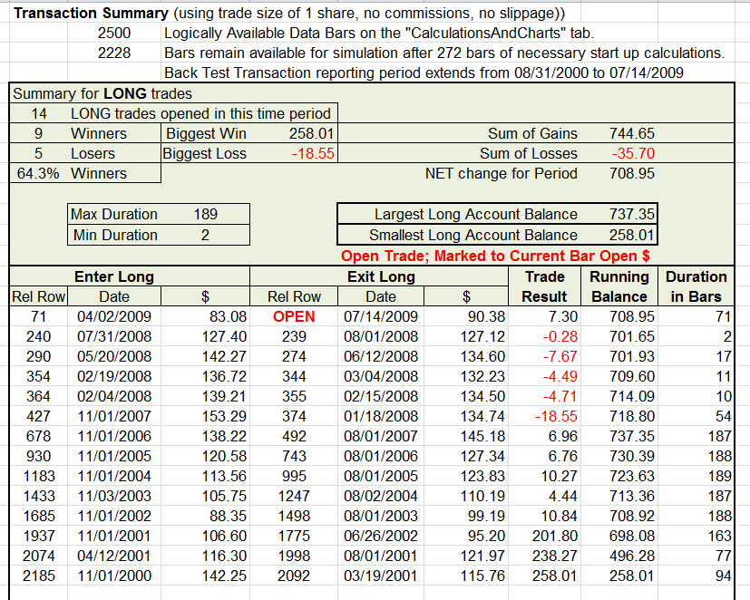
Replicating the performance tables included in Katsanos’ article were beyond the time available to create this spreadsheet. As a substitute, I have included a snapshot “trade summary” tab that incorporates all of the trades currently available on the ComputationsAndCharts tab. “Currently” as used here means that the trade summary reaches back approximately nine years in time from the “right-most bar” shown on the chart.
Figure 12 is a summary of the transactions selected by this system in a window ending on 7/14/2009 and stretching back to 8/31/2000. This is the same ending date as chart in Figure 1 and includes transactions that fall off the left edge of the chart.

FIGURE 12: EXCEL, TRADE SUMMARY, 2009–2000. This trade summary corresponds to Figure 1 above. Changing cell A11 changes that right-most bar and thus the window into SPY history.
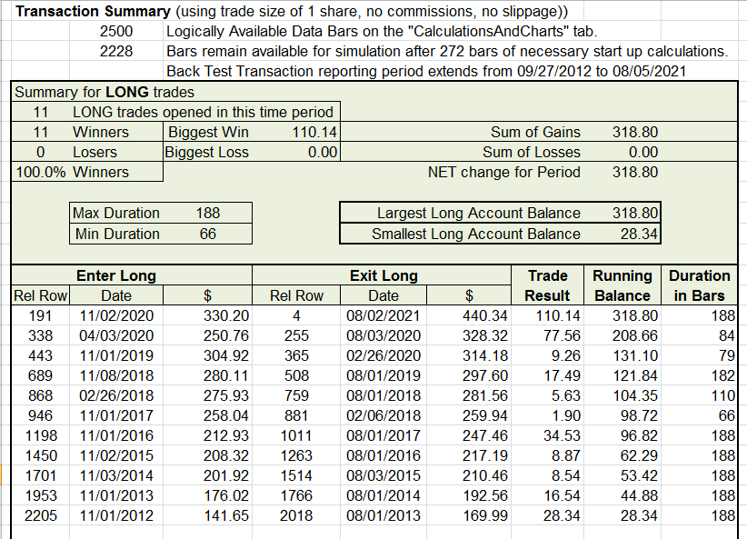
Figure 13 replicates Figure 7 from the article and looks at a more recent and wider window into SPY history. Figure 14 is the trade summary corresponding to the period displayed in Figure 3.

FIGURE 13: EXCEL. This replicates the article’s Figure 7 in Excel. It looks at a more recent and wider window into SPY history.

FIGURE 14: EXCEL, TRADE SUMMARY, 2012–2020. This shows a more recent nine-year trading window corresponding to Figure 13 above.
It will be interesting to test this with other symbols.
Note: I offer my apologies. There is a lot of computation involved in this spreadsheet along with a significant amount of VBA macro processing to produce the charts. That means that each change you make to user control numbers at the left or to the “show” buttons and boxes at the right will take a bit of time to complete. You may be “locked out” in that Excel may not respond to clicks or typing while this takes place. You may see a spinning cursor or even a flash of the charts during the lockout period.
To download this spreadsheet: The spreadsheet file for this Traders’ Tip can be downloaded here. To successfully download it, follow these steps:
- Right-click on the Excel file link, then
- Select “save as” (or “save target as”) to place a copy of the spreadsheet file on your hard drive.
—Ron McAllister
Excel and VBA programmer
rpmac_xltt@sprynet.com
BACK TO LIST
Originally published in the April 2022 issue of
Technical Analysis of STOCKS & COMMODITIES magazine.
All rights reserved. © Copyright 2022, Technical Analysis, Inc.
