TRADERS’ TIPS
June 2022

For this month’s Traders’ Tips, the focus is John F. Ehlers’ article in this issue, “Ehlers Loops, Part 1.” Here, we present the June 2022 Traders’ Tips code with possible implementations in various software.
You can right-click on any chart to open it in a new tab or window and view it at it’s originally supplied size, often much larger than the version printed in the magazine.
The Traders’ Tips section is provided to help the reader implement a selected technique from an article in this issue or another recent issue. The entries here are contributed by software developers or programmers for software that is capable of customization.

TradeStation: June 2022
In his article in this issue, “Ehlers Loops,” John Ehlers presents some concepts of price and volume relationship to determine if any predictive value can be obtained by the analysis. In the analysis, both price and volume are filtered using high-pass and low-pass filters with the result delivering the desired data wavelengths. The author suggests that the resulting Ehlers Loops are a way to discretionarily predict bullish and bearish moves that are based on the curvature and direction of rotation of motion in the price-volume chart.
The EasyLanguage given here creates an indicator that can be applied to a TradeStation chart to observe the plots versus price. Note that the code assumes that the export directory “C:\Temp” exists and that the indicator is applied to bar intervals of daily and above.
Indicator: TASC JUN 2022 Ehlers Loops
// TASC JUN 2022
// Ehlers Loops Part 1
// (C) 2005-2022 John F. Ehlers

// code is designed for Daily and above bar intervals
// since the keyword "Volume" is used for Volume

inputs:
	LPPeriod( 20 ),
	HPPeriod( 125 ),
	PriceRMSColor( Red ),
	ZeroLineColor( White ),
	VolRMSColor( Yellow );

variables:
	hpa1( 0 ),
	hpb1( 0 ),
	hpc1( 0 ),
	hpc2( 0 ),
	hpc3( 0 ),
	ssa1( 0 ),
	ssb1( 0 ),
	ssc1( 0 ),
	ssc2( 0 ),
	ssc3( 0 ),
	HP( 0 ),
	VolHP( 0 ),
	Price( 0 ),
	PriceMS( 0 ),
	PriceRMS( 0 ),
	Vol( 0 ),
	VolMS( 0 ),
	VolRMS( 0 );

if CurrentBar = 1 then
begin
	hpa1 = ExpValue( -1.414 * 3.14159 / HPPeriod );
	hpb1 = 2 * hpa1 * Cosine( 1.414 * 180/HPPeriod );
	hpc2 = hpb1;
	hpc3 = -hpa1 * hpa1;
	hpc1 = ( 1 + hpc2 - hpc3 ) / 4;
	ssa1 = ExpValue( -1.414 * 3.14159 / LPPeriod );
	ssb1 = 2 * ssa1 * Cosine( 1.414 * 180/LPPeriod );
	ssc2 = ssb1;
	ssc3 = -ssa1 * ssa1;
	ssc1 = 1 - ssc2 - ssc3;
end;

// Normalized Roofing Filter for Price
// 2 Pole Butterworth Highpass Filter
HP = hpc1 * ( Close - 2 * Close[1] + Close[2] )
 + hpc2 * HP[1] + hpc3 * HP[2];
if CurrentBar < 3 then
	HP = 0;

// Smooth with a Super Smoother Filter
Price = ssc1 * ( HP + HP[1] ) / 2 + ssc2 * Price[1]
 + ssc3 * Price[2];
if CurrentBar < 3 then
	Price = 0;

//Scale Price in terms of Standard Deviations
if CurrentBar = 1 then
	PriceMS = Price * Price
else
	PriceMS =.0242 * Price*Price + .9758 * PriceMS[1];

if PriceMS <> 0 then
	PriceRMS = Price / SquareRoot( PriceMS );

// Normalized Roofing Filter for Volume
// 2 Pole Butterworth Highpass Filter
VolHP = hpc1*( Volume - 2 * Volume[1] + Volume[2] ) +
 hpc2 * VolHP[1] + hpc3 * VolHP[2];
if CurrentBar < 3 then
	VolHP = 0;

// smooth with a Super Smoother Filter
Vol = ssc1 * ( VolHP + VolHP[1] ) / 2 + ssc2 * Vol[1]
 + ssc3 * Vol[2];
if CurrentBar < 3 then
	Vol = 0;

// scale Vol in terms of Standard Deviations
if CurrentBar = 1 then
	VolMS = Vol * Vol
else
	VolMS = .0242 * Vol * Vol + .9758 * VolMS[1];

if VolMS <> 0 then
	VolRMS = Vol / SquareRoot( VolMS );

// conventional plots
Plot1( PriceRMS, "PriceRMS", PriceRMSColor,
 default, 1 );
Plot2( 0, "Zero", ZeroLineColor, default, 0 );
Plot3( VolRMS, "VolRMS", VolRMSColor, default, 1 );

// output to text file
// ensure c:\Temp directory exists
print( File( "c:\Temp\EhlersLoops.csv" ), Date, ",",
 VolRMS, ",", PriceRMS );
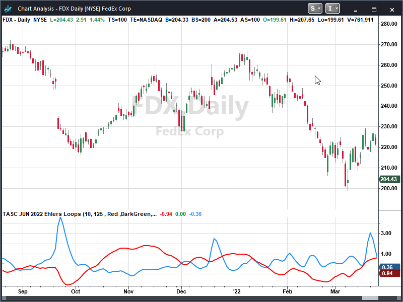
A sample chart is shown in Figure 1.

FIGURE 1: TRADESTATION. Demonstrated here is an indicator that can be applied to a TradeStation chart to observe the plots versus price.
This article is for informational purposes. No type of trading or investment recommendation, advice, or strategy is being made, given, or in any manner provided by TradeStation Securities or its affiliates.
—Chris Imhof
TradeStation Securities, Inc.
www.TradeStation.com
BACK TO LIST

TradingView: June 2022
Here is the Pine Script code for TradingView that implements the Ehlers Loops introduced by John Ehlers in his article in this issue.
//  TASC Issue: June 2022 - Vol. 40, Issue 7
//     Article: Ehlers Loops
//  Article By: John F. Ehlers
//    Language: TradingView's Pine Script v5
// Provided By: PineCoders, for tradingview.com

//@version=5
indicator("TASC 2022.06 Ehlers Loops", "ELs", precision=3)

//== 2 Pole Butterworth Highpass Filter ==//
butterworthHP(float Series, float Period) =>
    var float ALPHA =  math.pi * math.sqrt(2.0) / Period
    var float BETA  =  math.exp(-ALPHA )
    var float COEF2 = -math.pow(BETA, 2)
    var float COEF1 =  math.cos( ALPHA ) * 2.0 * BETA
    var float COEF0 =  (1.0 + COEF1 - COEF2) * 0.25
    float tmp    = nz(Series[1],  Series)
    float whiten =    Series + nz(Series[2], tmp) - 2.0 * tmp
    float smooth = na, smooth := COEF0 *     whiten     +
                                 COEF1 *  nz(smooth[1]) +
                                 COEF2 *  nz(smooth[2])

//===== 2 Pole Super Smoother Filter =====//
superSmoother(float Series, float Period) =>
    var float ALPHA =  math.pi * math.sqrt(2.0) / Period
    var float BETA  =  math.exp(-ALPHA )
    var float COEF2 = -math.pow(BETA, 2)
    var float COEF1 =  math.cos( ALPHA ) * 2.0 * BETA
    var float COEF0 =  1.0 - COEF1 - COEF2
    float sma2   = math.avg(Series, nz(Series[1], Series))
    float smooth = na, smooth := COEF0 *      sma2      +
                                 COEF1 *  nz(smooth[1]) +
                                 COEF2 *  nz(smooth[2])

//===== Faster Root Mean Square =====//
fastRMS(float Series, float Period) =>
    if Period < 1
        runtime.error("Err: fastRMS(Period=) is less than 1")
    var float COEF0 = 2.0 / (Period + 1)
    var float COEF1 = 1.0 -  COEF0
    float pow = math.pow(Series, 2)
    float ema = na, ema := COEF0 *    pow +
                           COEF1 * nz(ema[1], pow)
    nz(Series / math.sqrt(ema))

source    = input.source(close,      "Source")
periodLP  = input.int( 20,  "Low-Pass Period", minval= 7)
periodHP  = input.int(125, "High-Pass Period", minval=20)
periodRMS = input.int( 80,       "RMS Period",   step=10)

//==== Normalized Roofing Filter for Price ====//
float HP       = butterworthHP(source, periodHP )
float Price    = superSmoother(    HP, periodLP )
float PriceRMS =       fastRMS( Price, periodRMS)

//=== Normalized Roofing Filter for Volume ==//
float VolHP  = butterworthHP(volume, periodHP )
float Vol    = superSmoother( VolHP, periodLP )
float VolRMS =       fastRMS(   Vol, periodRMS)

plot(PriceRMS, "Area", #0077FF40, style=plot.style_area)
plot(PriceRMS, "PRMS", #0077FF, 2)
plot(  VolRMS, "VRMS", #FF7700)

hline(    2.0,   "2σ", #FF0000CC)
hline(    1.0,   "1σ", #FF000055, hline.style_dotted, 2)
hline(    0.0, "Zero", #808080)
hline(   -1.0,  "-1σ", #00FF0055, hline.style_dotted, 2)
hline(   -2.0,  "-2σ", #00FF00CC)
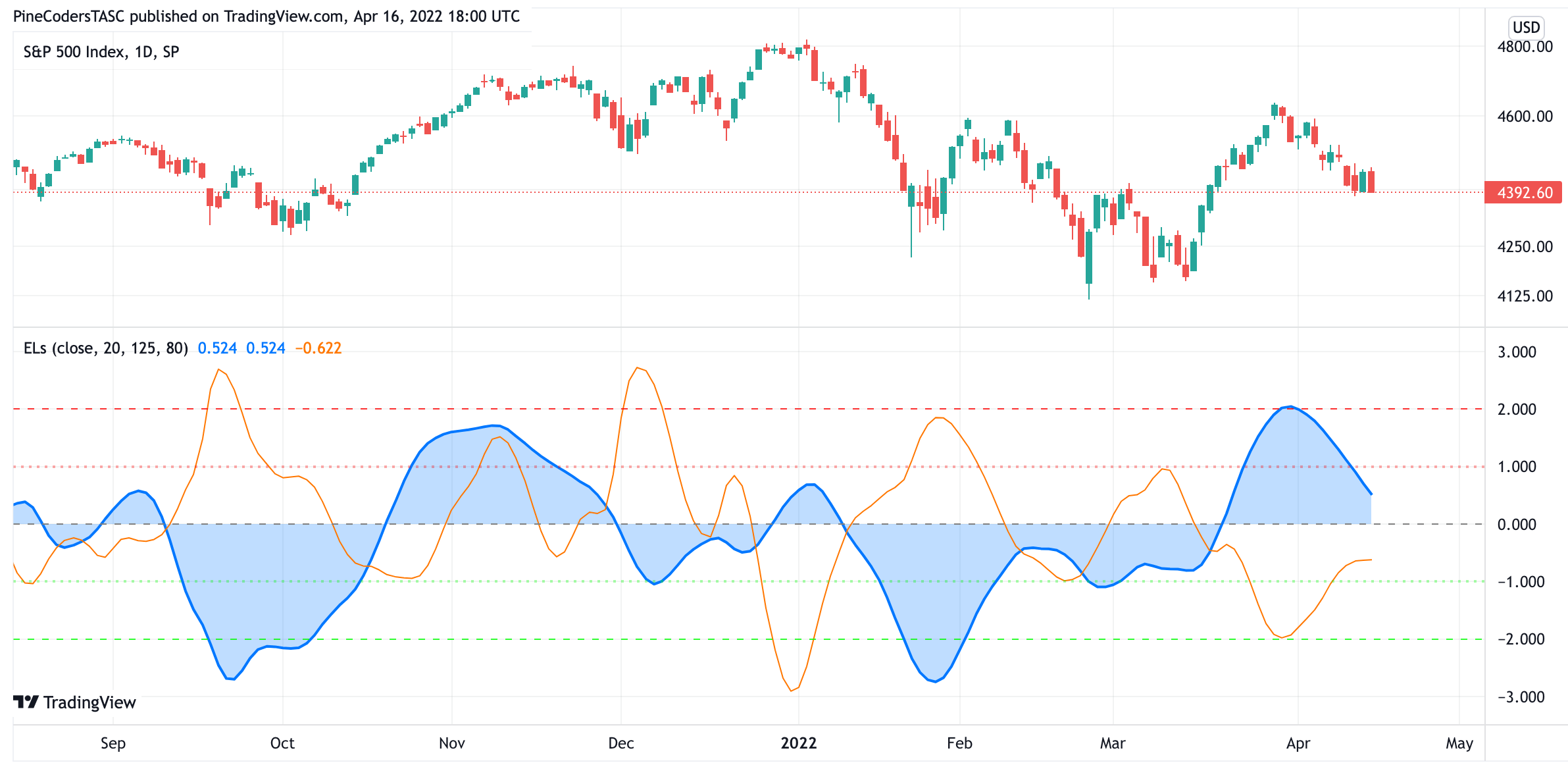
An example chart is shown in Figure 2.

FIGURE 2: TRADINGVIEW. Here are Ehlers Loops implemented on a chart by TradingView.
—PineCoders, for TradingView
www.TradingView.com
BACK TO LIST

Wealth-Lab.com: June 2022
In his article in this issue, John Ehlers brings in his expertise in digital signal processing to introduce an unusual way of analyzing the price/volume relationships. For discretionary traders, his Ehlers Loops open up a new method to see ahead potential bullish and bearish moves based on the curvature and direction of rotation of motion as a function of time in the price-volume chart.
Wealth-Lab 8 makes it easy to display the various custom plots like line or bar charts, pie graphs, and scatter plots with a few lines of code. The code below accomplishes this with an open-source plotting library for .NET called ScottPlot.
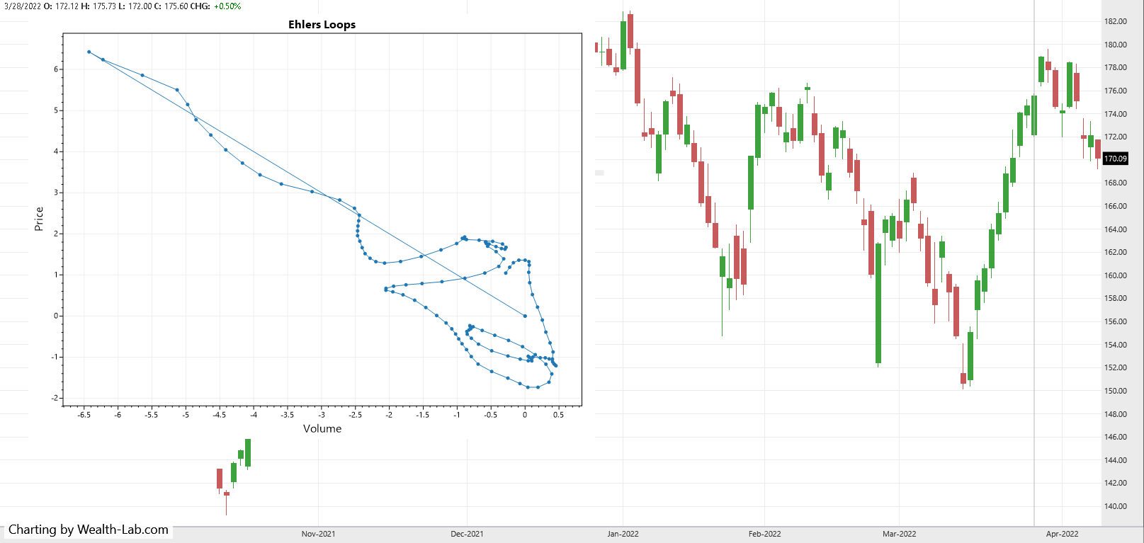
A Wealth-Lab chart showing Ehlers Loops superimposed on Apple is shown in Figure 3.

FIGURE 3: WEALTH-LAB. Here, Ehlers Loops are superimposed on a chart of Apple (AAPL) in Wealth-Lab 8.
using WealthLab.Backtest;
using System;
using WealthLab.Core;
using WealthLab.Indicators;
using System.Drawing;
using System.Collections.Generic;
using ScottPlot;

namespace WealthScript1
{
	public class TASC202206EhlersLoops : UserStrategyBase
	{
		/* create indicators and other objects here, this is executed prior to the main trading loop */
		public override void Initialize(BarHistory bars)
		{
			int LPPeriod = 20, HPPeriod = 125;
			double Deg2Rad = Math.PI / 180.0;
			List<double> lstDates = new List<double>();
			List<double> lstValuesP = new List<double>();
			List<double> lstValuesV = new List<double>();

			hpa1 = Math.Exp(-1.414 * Math.PI / HPPeriod);
			hpb1 = 2.0 * hpa1 * Math.Cos((1.414 * 180d / HPPeriod) * Deg2Rad);
			hpc2 = hpb1;
			hpc3 = -hpa1 * hpa1;
			hpc1 = (1 + hpc2 - hpc3) / 4;
			ssa1 = Math.Exp(-1.414 * Math.PI / LPPeriod);
			ssb1 = 2.0 * ssa1 * Math.Cos((1.414 * 180d / LPPeriod) * Deg2Rad);
			ssc2 = ssb1;
			ssc3 = -ssa1 * ssa1;
			ssc1 = 1 - ssc2 - ssc3;

			/* 2 Pole Butterworth Highpass Filter */
			TimeSeries HP = new TimeSeries(bars.DateTimes, 0);
			for (int i = 2; i < bars.DateTimes.Count; i++)
			{
				HP[i] = hpc1 * (bars.Close[i] - 2 * bars.Close[i - 1] + bars.Close[i - 2]) + hpc2 * HP[i - 1] + hpc3 * HP[i - 2];
			}

			/* Smooth with a Super Smoother Filter */
			TimeSeries Price = new TimeSeries(bars.DateTimes, 0);
			for (int i = 2; i < bars.DateTimes.Count; i++)
			{
				Price[i] = ssc1 *(HP[i] + HP[i - 1]) / 2 + ssc2 *Price[i - 1] + ssc3 *Price[i - 2];
			}

			/* Scale Price in terms of Standard Deviations */
			TimeSeries PriceMS = new TimeSeries(bars.DateTimes, 0);
			TimeSeries PriceRMS = new TimeSeries(bars.DateTimes, 0);
			for (int i = 0; i < bars.DateTimes.Count; i++)
			{
				if(i < 2)
					PriceMS[i] = Math.Pow(Price[i], 2);
				else
					PriceMS[i] = 0.0242 * Price[i] * Price[i] + 0.9758 * PriceMS[i - 1];
				if(PriceMS[i] != 0)
					PriceRMS[i] = Price[i] / Math.Sqrt(PriceMS[i]);

				lstValuesP.Add(PriceRMS[i]);
			}

			/* Normalized Roofing Filter for Volume */

			/* 2 Pole Butterworth Highpass Filter */
			TimeSeries VolHP = new TimeSeries(bars.DateTimes, 0);
			for (int i = 2; i < bars.DateTimes.Count; i++)
			{
				VolHP[i] = hpc1 * (bars.Volume[i] - 2 * bars.Volume[i - 1] + bars.Volume[i - 2]) + hpc2 * VolHP[i - 1] + hpc3 * VolHP[i - 2];
			}

			/* Smooth with a Super Smoother Filter */
			TimeSeries Vol = new TimeSeries(bars.DateTimes, 0);
			for (int i = 2; i < bars.DateTimes.Count; i++)
			{
				Vol[i] = ssc1 * (VolHP[i] + VolHP[i - 1]) / 2 + ssc2 * Vol[i - 1] + ssc3 * Vol[i - 2];
			}

			/* Scale Vol in terms of Standard Deviations */
			TimeSeries VolMS = new TimeSeries(bars.DateTimes, 0);
			TimeSeries VolRMS = new TimeSeries(bars.DateTimes, 0);
			for (int i = 0; i < bars.DateTimes.Count; i++)
			{
				lstDates.Add(i);

				if (i < 2)
					VolMS[i] = Math.Pow(Vol[i], 2);
				else
					VolMS[i] = 0.0242 * Vol[i] * Vol[i] + 0.9758 * VolMS[i - 1];

				if (VolMS[i] != 0)
					VolRMS[i] = Vol[i] / Math.Sqrt(VolMS[i]);

				lstValuesV.Add(VolRMS[i]);
			}


			Bitmap bmp = null;
			Plot plt = new ScottPlot.Plot(800, 600);
			plt.Title("Ehlers Loops");
			plt.YLabel("Price");
			plt.XLabel("Volume");

			plt.PlotScatter(lstValuesV.ToArray(), lstValuesP.ToArray());
			bmp = plt.GetBitmap();
			DrawImageAt(bmp, 40, 20);
		}

		/* execute the strategy rules here, this is executed once for each bar in the backtest history */
		public override void Execute(BarHistory bars, int idx)
		{
		}

		/* declare private variables below */
		double hpa1, hpb1, hpc2, hpc3, hpc1, ssa1, ssb1, ssc2, ssc3, ssc1;
	}
}
—Gene Geren (Eugene)
Wealth-Lab team
www.wealth-lab.com
BACK TO LIST

NinjaTrader: June 2022
The Ehlers Loops indicator, which is introduced in the article in this issue by John Ehlers titled “Ehlers Loops,” is available for download at the following links for NinjaTrader 8 and for NinjaTrader 7:
Once the file is downloaded, you can import the indicator into NinjaTrader 8 from within the control center by selecting Tools → Import → NinjaScript Add-On and then selecting the downloaded file for NinjaTrader 8. To import into NinjaTrader 7, from within the control center window, select the menu File → Utilities → Import NinjaScript and select the downloaded file.
You can review the indicator’s source code in NinjaTrader 8 by selecting the menu New → NinjaScript Editor → Indicators from within the control center window and selecting the “Ehlers Loops” file. You can review the indicator’s source code in NinjaTrader 7 by selecting the menu Tools → Edit NinjaScript → Indicator from within the control center window and selecting the “Ehlers Loops” file.
NinjaScript uses compiled DLLs that run native, not interpreted, which provides you with the highest performance possible.
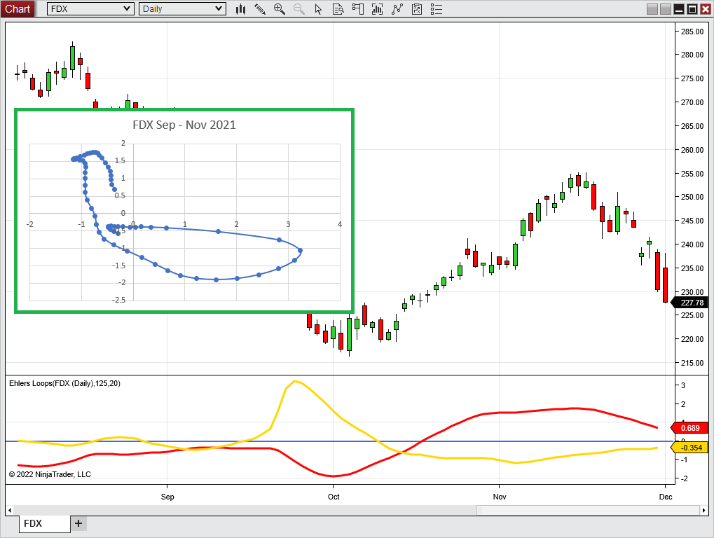
A chart displaying the indicator is shown in Figure 4.

FIGURE 4: NINJATRADER. This shows an example of an Ehlers Loop of FedEx (FDX) for three months in 2021. The loop plot starts on September 1.
—Kate Windheuser
NinjaTrader, LLC
www.ninjatrader.com
BACK TO LIST

Neuroshell Trader: June 2022
Ehlers Loops, which are introduced by John Ehlers in his article in this issue, can be easily computed in NeuroShell Trader using NeuroShell Trader’s ability to call external dynamic linked libraries. Dynamic linked libraries can be written in C, C++, or Power Basic.
After moving the code given in the article to your preferred compiler and creating a DLL, you can insert the resulting indicator as follows:
- Select “new indicator” from the insert menu.
- Choose the External Program & Library Calls category.
- Select the appropriate External DLL Call indicator.
- Set up the parameters to match your DLL.
- Select the finished button.
Once the values for price and volume are on the chart, simply use NeuroShell Trader’s export feature to export the values to an Excel spreadsheet as described in the article.
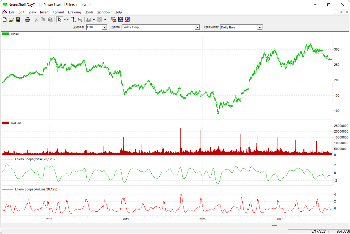
An example chart is shown in Figure 5.

FIGURE 5: NEUROSHELL TRADER. This NeuroShell Trader chart shows the calculated Ehlers Loops values for Fedex.
NeuroShell Trader users can go to the Stocks & Commodities section of the NeuroShell Trader free technical support website to download a copy of this or any previous Traders’ Tips.
—Ward Systems Group, Inc.
sales@wardsystems.com
www.neuroshell.com
BACK TO LIST

The Zorro Project: June 2022
Price charts normally display price over time, or maybe, in some cases with special bars, price over momentum. In his article in this issue, John Ehlers proposes to display price over volume in a scatter plot. The result is a special curve, which the author calls an “Ehlers Loop,” that is considered by the author to have predictive value. For this purpose, Ehlers filters the low and high frequencies out of the volume and price data with a roofing filter.
Here is the C code converted from the EasyLanguage given in the article:
var Roofing(var *Data,int HPeriod,int LPeriod)
{
  var f = 1.414*PI/HPeriod;
  var hpa1 = exp(-f);
  var hpc2 = 2*hpa1*cos(f/2);
  var hpc3 = -hpa1*hpa1;
  var hpc1 = (1 + hpc2 - hpc3) / 4;
  f = 1.414*PI/LPeriod;
  var ssa1 = exp(-f);
  var ssc2 = 2*ssa1*cos(f/2);
  var ssc3 = -ssa1*ssa1;
  var ssc1 = 1 - ssc2 - ssc3;

  vars HP = series(Data[0],3);
  HP[0] = hpc1*(Data[0] - 2*Data[1] + Data[2]) + hpc2*HP[1] + hpc3*HP[2];
  vars SS = series(HP[0],3);
  SS[0] = ssc1*(HP[0] + HP[1])/2 + ssc2*SS[1] + ssc3*SS[2];
  var Scaled = EMA(SS[0]*SS[0],.0242);
  return SS[0]/sqrt(Scaled);
}
Now we only need to apply that filter to the price and volume series. The filtered data points serve as XY coordinates for our curve—the “Ehlers Loop.” In his article, Ehlers exports the data to Excel in order to draw the scatter plot. However, Zorro is capable of drawing scatter plots within the platform.
The following script reads three months of stock data from an online source and displays it as an Ehlers Loop:
function run()
{
  StartDate = ymd(wdate(NOW)-90); // 90 days before today
  BarPeriod = 1440;
  asset("FDX");
  var PriceRMS = Roofing(seriesC(),125,20);
  var VolRMS = Roofing(series(marketVol()),125,20);

  if(is(LOOKBACK)) return;  // don't plot the lookback period
  plotGraph("Loop",VolRMS,PriceRMS,DOT|GRAPH,BLUE);
  plotGraph("Loops",VolRMS,PriceRMS,SPLINE|GRAPH,TRANSP|GREY);
  if(is(EXITRUN))
    plotGraph("Last",VolRMS,PriceRMS,SQUARE|GRAPH,RED);
}
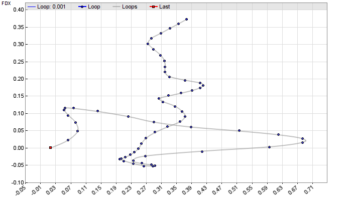
The plotGraph function is used to display each coordinate with a blue dot and connect the dots with spline lines. The last day is marked with a red square. Shown in Figure 6 is an Ehlers Loop of FDX on April 13, 2022.

FIGURE 6: ZORRO PROJECT. Shown here is an Ehlers Loop plotted on FedEx (FDX) on April 13, 2022. To draw the Ehlers Loops in Zorro, the plotGraph function is used to display each coordinate with a blue dot and connect the dots with spline lines. The last day is marked with a red square.
Ehlers intended his loops for discretionary trading, but it could also be automated. For instance, the last N coordinates could be used as inputs for Zorro’s neural net, which can then be trained to predict tomorrow’s price. Or even simpler, the slope at the last point—the red square—could trigger a buy order when positive or a sell order when negative. I leave to the reader to experiment with a trading system.
The scripts for the roofing indicator and the Ehlers Loop can be downloaded from the 2022 script repository on https://financial-hacker.com. The Zorro software can be downloaded from https://zorro-project.com.
—Petra Volkova
The Zorro Project by oP group Germany
https://zorro-project.com
BACK TO LIST
Microsoft Excel: June 2022
In his article in this issue, John Ehlers introduces a technique of plotting price and volume that he calls “Ehlers Loops.” The computations to generate Ehlers Loops are straightforward. Figure 7 replicates in Excel the chart from his article giving an example of an Ehlers Loop on FedEx (FDX).

FIGURE 7: EXCEL. This chart replicates in Excel the chart of Ehlers Loops from John Ehlers’ article in this issue.
Getting Excel 2010 to put date data labels on the points of the loop chart is a significant problem that newer versions of Excel can handle easily. So a different approach is necessary for this spreadsheet.
To assist visualizing clockwise or counter-clockwise flows, I have opted to connect the loop data points with arrows to indicate the forward-in-time point-to-point progression along the loop.
Next, I am using a red circle as my cursor location along the loop to indicate the loop point that corresponds with the price and volume bars under their respective chart cursors.
The legend entry in the upper right of the loop chart displays the date of the point under the circle.
All of the chart cursors are controlled by the slider below the volume chart. (See Figure 8.) You may find it interesting to play with the slider to get a better feel for what the Ehlers Loop is telling us about the price and volume action.

FIGURE 8: EXCEL. You can see the coordination of the price and the volume chart cursors with the red circle indicating the corresponding point along the loop.
Figure 9 demonstrates that the loop chart can, as John Ehlers noted, get rather messy. To create Figure 9 I merely moved the charting data window forward by 92 days (setting A11 to zero) and plotted the same number of bars. Reducing the cell A12 (data points to plot) value can help to reduce the congestion.

FIGURE 9: EXCEL. Here, the data window was shifted 92 bars forward in time by changing cell A11 to zero in order to reduce clutter.
For completeness, Figure 10 includes plots of the raw volume RMS (root mean square) and price RMS values that are used as the X and Y coordinates to generate the loops chart.

FIGURE 10: EXCEL. This example includes plots of the raw volume RMS (root mean square) and price RMS values that are used as the X and Y coordinates to generate the loops chart.
To download this spreadsheet: The spreadsheet file for this Traders’ Tip can be downloaded here. To successfully download it, follow these steps:
- Right-click on the Excel file link, then
- Select “save as” (or “save target as”) to place a copy of the spreadsheet file on your hard drive.
Error notice: A reader emailed me to let me know that the April 2022 issue spreadsheet contains an error in column “H” on the “transaction summary” tab that causes incorrect individual transaction results and skews the totals.
The formulas in cells H27:H380 are incorrect. The formulas in cell H26 and above are correct.
The quick fix is to drag-fill cell H26 down over cells H27:H380. Here is a review of how to do that:
Click on cell H26. This places a black outline around cell H26 with a small black square in the lower right of that outline. Hover your cursor over that small black square until your cursor changes to a cross without arrow heads. Left-click and hold. While holding the left-click, drag your cursor down the H column to cell H380. Then save the corrected spreadsheet.
—Ron McAllister
Excel and VBA programmer
rpmac_xltt@sprynet.com
BACK TO LIST

TradersStudio: June 2022
The importable TradersStudio file based on John Ehlers’ article, “Ehlers Loops” can be obtained on request via email to info@TradersEdgeSystems.com. The code is also shown below.
Code for the author’s indicators is provided in following files:
- Function EHLERS_LOOPS: computes Elegant Oscillator indicator
- Indicator plot EHLERS_LOOPS_IND: plots the Elegant Oscillator indicator on a chart
'Ehlers Loops, TASC June 2022
'Author: John F. Ehlers
'Coded by: Richard Denning, 4/20/2022
'Ehlers Loops
'(C) 2005-2022 John F. Ehlers

Function EHLERS_LOOPS(LPPeriod, HPPeriod, ByRef PriceRMS )
'LPPeriod = 20
'HPPeriod = 125
    Dim hpa1 As BarArray
    Dim hpb1 As BarArray
    Dim hpc1 As BarArray
    Dim hpc2 As BarArray
    Dim hpc3 As BarArray
    Dim ssa1 As BarArray
    Dim ssb1 As BarArray
    Dim ssc1 As BarArray
    Dim ssc2 As BarArray
    Dim ssc3 As BarArray
    Dim HP As BarArray
    Dim VolHP As BarArray
    Dim Price As BarArray
    Dim PriceMS As BarArray
    'Dim PriceRMS As BarArray
    Dim VolR As BarArray
    Dim VolMS As BarArray
    Dim VolRMS As BarArray
    If BarNumber=FirstBar Then
        hpa1 = TStation_ExpValue(-1.414*3.14159 / HPPeriod)
        hpb1 = 2*hpa1*TStation_Cosine(1.414*180 / HPPeriod)
        hpc2 = hpb1
        hpc3 = -hpa1*hpa1
        hpc1 = (1 + hpc2 - hpc3) / 4
        ssa1 = TStation_ExpValue(-1.414*3.14159 / LPPeriod)
        ssb1 = 2*ssa1*TStation_Cosine(1.414*180 / LPPeriod)
        ssc2 = ssb1
        ssc3 = -ssa1*ssa1
        ssc1 = 1 - ssc2 - ssc3
    End If
    HP = hpc1*(Close - 2*Close[1] + Close[2]) + hpc2*HP[1] + hpc3*HP[2]
    If BarNumber=FirstBar Then
        HP = 0
    End If
    Price = ssc1*(HP + HP[1]) / 2 + ssc2*Price[1] + ssc3*Price[2]
    If BarNumber=FirstBar Then
        Price = 0
    End If
    If BarNumber=FirstBar Then
        PriceMS = Price*Price
    Else
        PriceMS = 0.0242*Price*Price + 0.9758*PriceMS[1]
    End If
    If PriceMS <> 0 Then
        PriceRMS = Price / Sqr(PriceMS)
    End If

    VolHP = hpc1*(Vol - 2*Vol[1] + Vol[2]) + hpc2*VolHP[1] + hpc3*VolHP[2]
    If BarNumber=FirstBar Then
        VolHP = 0
    End If
    VolR = ssc1*(VolHP + VolHP[1]) / 2 + ssc2*VolR[1] + ssc3*VolR[2]
    If BarNumber=FirstBar Then
        VolR = 0
    End If
    If BarNumber=FirstBar Then
        VolMS = VolR*VolR
    Else
        VolMS = 0.0242*VolR*VolR + 0.9758*VolMS[1]
    End If
    If VolMS <> 0 Then
        VolRMS = VolR / Sqr(VolMS)
    End If

    'Print(File("c:\Temp\EhlersLoops.csv"), FormatDateTime(Date), ",", VolRMS, ",", PriceRMS)
    Print FormatDateTime(Date), ",", Round(VolRMS,4), ",", Round(PriceRMS,4)
EHLERS_LOOPS = VolRMS
End Function
'---------------------------------------------------------------------------------------------
'INDICATOR PLOT:
'Ehlers Loops, TASC June 2022
'Author: John F. Ehlers
'Coded by: Richard Denning, 4/20/2022
'Ehlers Loops
'(C) 2005-2022 John F. Ehlers

Sub EHLERS_LOOPS_IND(LPPeriod, HPPeriod)
'LLPeriod = 20, HPPeriod = 125
Dim PriceRMS As BarArray
Dim VolRMS As BarArray

VolRMS = EHLERS_LOOPS(LPPeriod, HPPeriod, PriceRMS)
Plot1(PriceRMS)
Plot2(VolRMS)
End Sub
'---------------------------------------------------
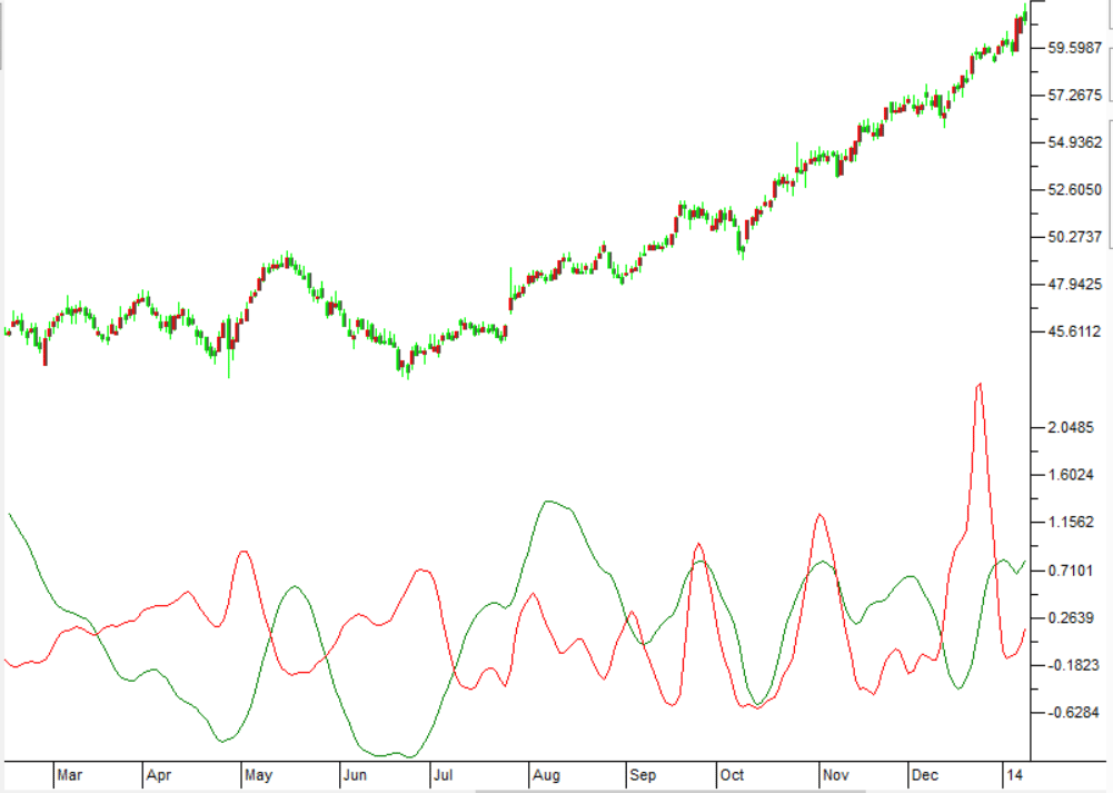
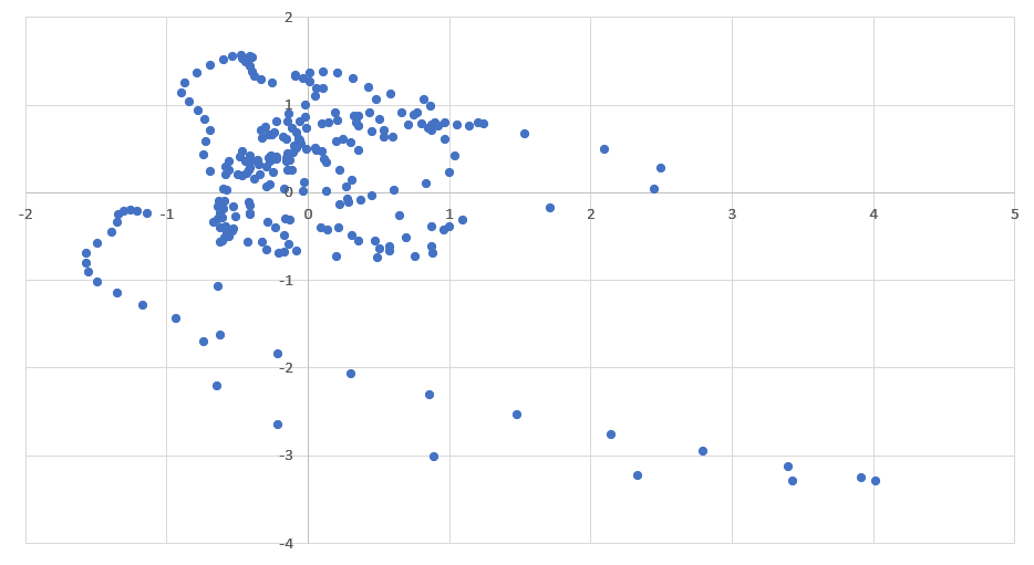
Figure 11 shows the indicator on a conventional chart of Verisign (VRSN) during 2013. Figure 12 is a scatter plot using data from the terminal window and pasting into Excel where the plot was created.

FIGURE 11: TRADERSSTUDIO. This shows an example of the Ehlers Loops indicator on a conventional chart of Verisign (VRSN) during 2013.

FIGURE 12: TRADERSSTUDIO. This shows the Ehlers Loops indicator on a scatter plot of Verisign (VRSN) during part of 2013 and 2014.
—Richard Denning
info@TradersEdgeSystems.com
for TradersStudio
BACK TO LIST
Originally published in the June 2022 issue of
Technical Analysis of STOCKS & COMMODITIES magazine.
All rights reserved. © Copyright 2022, Technical Analysis, Inc.
