TRADERS’ TIPS
April 2023
For this month’s Traders’ Tips, the focus is John Ehlers’ article in this issue, “Just Ignore Them.” Here, we present the April 2023 Traders’ Tips code with possible implementations in various software.
You can right-click on any chart to open it in a new tab or window and view it at it’s originally supplied size, often much larger than the version printed in the magazine.
The Traders’ Tips section is provided to help the reader implement a selected technique from an article in this issue or another recent issue. The entries here are contributed by software developers or programmers for software that is capable of customization.

TradeStation: April 2023
In his article in this issue, “Just Ignore Them: Undersampling The Data As A Smoothing Technique,” John Ehlers explains that data smoothing is often used as a means to help avoid trading whipsaws. While this can result in fewer trading signals, it can also result in a lag in those trading signals. In the article, Ehlers describes how undersampling coupled with Hann-windowed finite impulse response (FIR) filters can be used to remove high-frequency components in price data, resulting in less lag than that of traditional smoothing filters.
Function: $Hann

{
	TASC APR 2023
	Function: Hann Windowed Lowpass FIR Filter
	(c) 2021-2022 John F. Ehlers
}
inputs:
	Price( numericseries ),
	Length( numericsimple );

variables:
	Count( 0 ),
	Coef( 0 ),
	Filt( 0 );

Filt = 0;
Coef = 0;

for Count = 1 to Length
begin
	Filt = Filt + (1 - Cosine(360 * Count / (Length +
	 1))) * Price[Count - 1];
	Coef = Coef +
	 (1 - Cosine(360 * Count / (Length + 1)));
end;

if Coef <> 0 Then
	$Hann = Filt / Coef;


Indicator: Undersampled Double MA

{
	TASC APR 2023
	Undersampled Double MA Indicator
	(c) 2022 John F. Ehlers
}

inputs:
	FastLength( 6 ),
	SlowLength( 12 );

variables:
	Sample( 0 ),
	FastAvg( 0 ),
	SlowAvg( 0 );

Sample = Sample[1];

//Sample every five days
if CurrentBar / 5 = IntPortion(CurrentBar / 5) then
	Sample = Close;
//Find Fast Average using Hann FIR filter
FastAvg = $Hann(Sample, FastLength);
//Find Slow Average using Hann FIR filter
SlowAvg = $Hann(Sample, SlowLength);

Plot1(FastAvg, "FastAvg");
Plot2(SlowAvg, "SlowAvg");


Indicator: Undersampled Intraday Double MA

{
	TASC APR 2023
	Undersampled Intraday Double MA Indicator
	(c) 2022 John F. Ehlers
}

inputs:
	BegDate( 1221117 ),
	FastLength( 20 ),
	SlowLength( 40 );

variables:
	Gap(0 ),
	Degap( 0 ),
	FastAvg( 0 ),
	SlowAvg( 0 );
	Degap = Degap[1];

if Time = 645 then
begin
	Gap = Close - Degap[1];
	Degap = Close - Gap;
end;

if Time = 800 or Time = 900
 or Time = 1000 or Time = 1100
 or Time = 1200 or Time = 1315 then
 	Degap = Close - Gap;

if Date < BegDate then
	Degap = Close;
//Find Fast Average using Hann FIR filter
FastAvg = $Hann(Degap, FastLength);
//Find Slow Average using Hann FIR filter
SlowAvg = $Hann(Degap, SlowLength);

Plot1(FastAvg, "Fast Avg");
Plot2(SlowAvg, "Slow Avg");
A sample chart is shown in Figure 1.
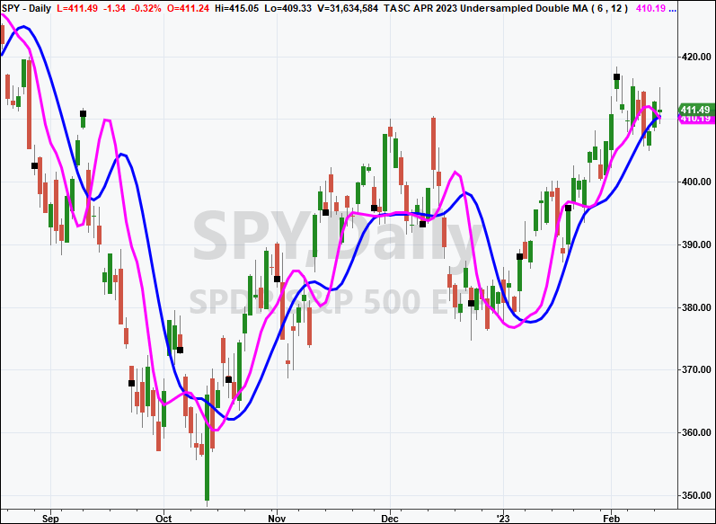
FIGURE 1: TRADESTATION. This TradeStation daily chart of the S&P 500 ETF SPY shows a portion of 2022 and 2023 with the undersampled double MA indicator applied. A fast length of 6 is used and a slow length of 12 is used. The fast average is shown in magenta and the slow average is shown in blue.
This article is for informational purposes. No type of trading or investment recommendation, advice, or strategy is being made, given, or in any manner provided by TradeStation Securities or its affiliates.
—John Robinson
TradeStation Securities, Inc.
www.TradeStation.com
BACK TO LIST

Wealth-Lab.com: April 2023
In his article “Just Ignore Them” in this issue, John Ehlers suggests a smoothing method by undersampling the data and using Hann windowing.
The Hann indicator is ready for use in Wealth-Lab 8, allowing the user to choose whether to apply undersampling to the data or leave it as is. You can apply it equally using various tools in Wealth-Lab such as Building Blocks (to create no-code trading strategies), the Indicator Profiler (which tells how much of an edge an indicator provides), or our Strategy Optimizer.
With Wealth-Lab’s ability to combine different indicators in a GUI wizard, Hann filters can even be used as a “smoother” to your favorite indicator like MFI, RSI, or momentum. The techniques, common to moving average interpretation, apply here as well.
Prototyping a trading system, including complex ideas, doesn’t take much effort with the Building Blocks feature. If you’re not familiar with Wealth-Lab, our web-based backtesting engine is free to use. Create a system (for example, applying the Hann filter to a price or indicator of choice) in its user-friendly interface and run backtests of your strategy right in the browser. As a natural next step, your strategy becomes instantly available in the Wealth-Lab desktop application for in-depth use. And if the strategy turns out to be good enough, you could choose to publish it for the benefit of the Wealth-Lab community of members. Strategies published by community members can be found at https://www.wealth-lab.com/Strategy/PublishedStrategies.
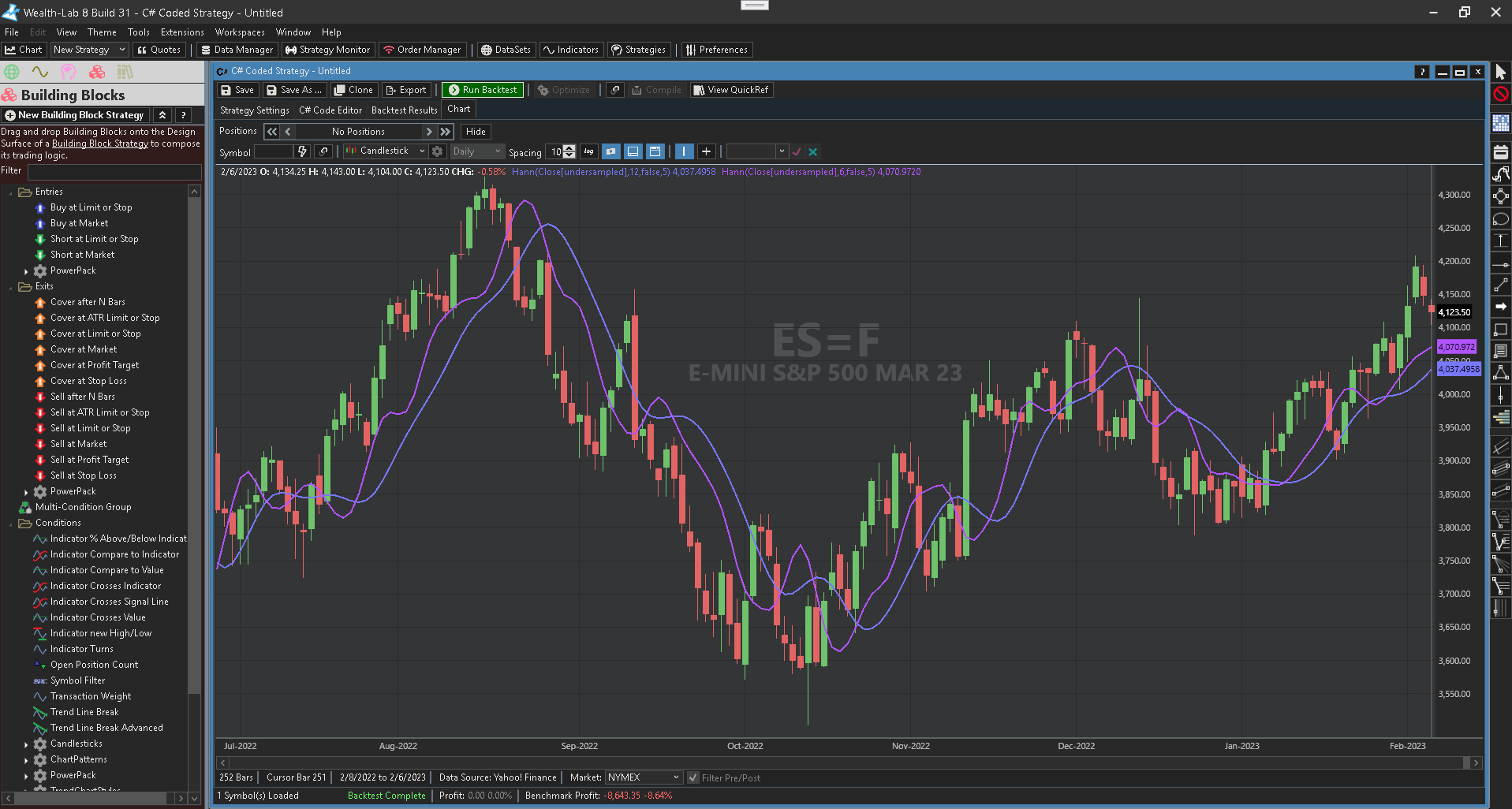
FIGURE 2: WEALTH-LAB. This sample chart demonstrates a 6- and 12-period Hann filter (5-period undersampled) on the daily chart of the emini S&P 500 futures (ES=F). Data provided by Yahoo! Finance.
—Gene Geren (Eugene)
Wealth-Lab team
www.wealth-lab.com
BACK TO LIST

NinjaTrader: April 2023
The smoothing technique that John Ehlers presents in his article in this issue, “Just Ignore Them,” using undersampling and Hann windowing is available for download from the following links for NinjaTrader 8 and for NinjaTrader 7:
Once the file is downloaded, you can import the indicator into NinjaTrader 8 from within the control center by selecting Tools → Import → NinjaScript Add-On and then selecting the downloaded file for NinjaTrader 8. To import into NinjaTrader 7, from within the control center window, select the menu File → Utilities → Import NinjaScript and select the downloaded file.
You can review the indicator’s source code in NinjaTrader 8 by selecting the menu New → NinjaScript Editor → Indicators from within the control center window and selecting the file you wish to examine. You can review the indicator’s source code in NinjaTrader 7 by selecting the menu Tools → Edit NinjaScript → Indicator from within the control center window and selecting the file to examine.
NinjaScript uses compiled DLLs that run native, not interpreted, which provides you with the highest performance possible.
A sample chart displaying the double moving average as discussed in Ehlers’ article is shown in Figure 3.
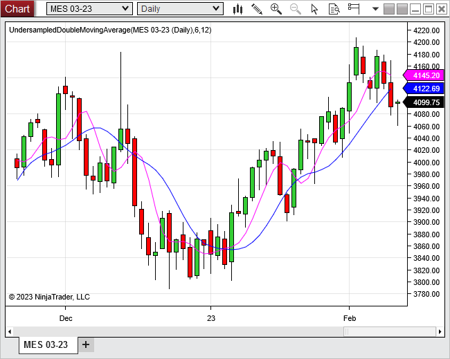
FIGURE 3: NINJATRADER. This shows an example of the undersampled double moving average on a daily chart of the emini ES, 11/15/2022 to 2/10/2023.
—Chelsea Bell
NinjaTrader, LLC
www.ninjatrader.com
BACK TO LIST

TradingView: April 2023
Here is TradingView Pine Script code implementing the undersampled double moving average indicator described in the article in this issue by John Ehlers, titled “Just Ignore Them: Undersampling The Data As A Smoothing Technique.”
//  TASC Issue: April 2023 - Vol. 41, Issue 5
//     Article: Undersampling The Data As A Smoothing Technique.
//              Just Ignore Them.
//  Article By: John Ehlers
//    Language: TradingView's Pine Script™ v5
// Provided By: PineCoders, for tradingview.com

//@version=5
string title  = 'TASC 2023.04 Undersampled Double MA'
string stitle = 'UDMA'
indicator(title, stitle, true)

// @function Samples a source every period of bars.
// @param period int   . Period of sampling.
// @param source float . Data source.
// @returns float.
sampledSource (int period = 5, float source = close) =>
   var float sample = source
   // sample every period:
   if bar_index % period == 0
       sample := source
   sample

// @function Hann Windowed Lowpass FIR Filter.
// @param source float . Data source.
// @param length int   . Length period.
// @returns float.
hann (float source, int length) =>
   float PIx2 = math.pi * 2.0, filt = 0.0, coef = 0.0
   for count = 1 to length
       float w = 1.0-math.cos(PIx2*count / (length + 1.0))
       filt += w * nz(source[count - 1])
       coef += w
   float hann = coef != 0.0 ? filt / coef : na
   hann

// @function Undersampled Double Moving Average.
// @param length       int   . Length period.
// @param samplePeriod int   . Sampling period.
// @param source       float . Data source.
// @returns float.
udma (int length      =     6,
int      samplePeriod =     5,
float    source       = close
) =>
   float sample = sampledSource(samplePeriod, source)
   //find average using Hann FIR filter:
   float result = hann(sample, length)
   result

int samplePeriod = input.int( 5, 'Sampling period:', 1)
int fastLength   = input.int( 6, 'Fast period:', 1)
int slowLength   = input.int(12, 'Slow period:', 1)

float fast = udma(fastLength, samplePeriod)
float slow = udma(slowLength, samplePeriod)

plot(fast, 'Fast UDMA', color.red, 4)
plot(slow, 'Slow UDMA', color.navy, 4)
The indicator is available on TradingView from the PineCodersTASC account at:
https://www.tradingview.com/u/PineCodersTASC/#published-scripts.
An example chart is shown in Figure 4.
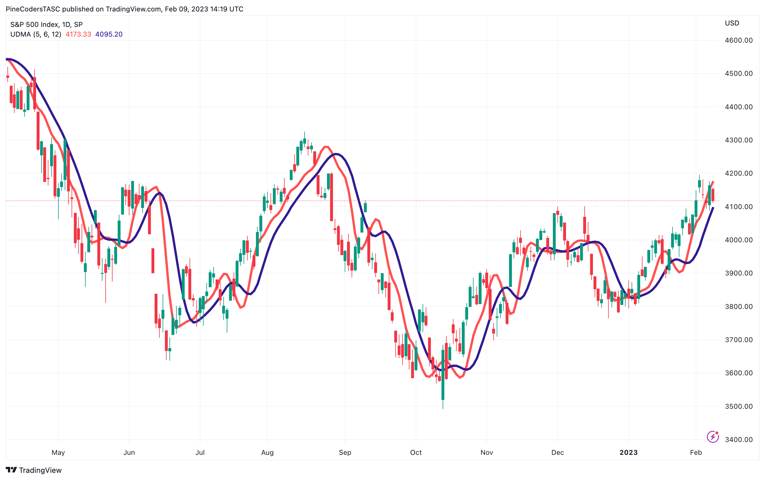
FIGURE 4: TRADINGVIEW. This daily TradingView chart of the S&P 500 index demonstrates the undersampled double moving average (5,6,12).
—PineCoders, for TradingView
www.TradingView.com
BACK TO LIST

NeuroShell Trader: April 2023
Using undersampling of the data as a smoothing technique, as described by John Ehlers in his article in this issue, “Just Ignore Them,” can be easily implemented in NeuroShell Trader by combining some of NeuroShell Trader’s 800+ indicators. To implement the undersampled intraday double MA indicator, select “new indicator” from the insert menu, and use the indicator wizard to set up the following indicators:
Gap	Sub(DayOpen(Date,Open,0),DayClose(Date,Close,1))
CumGap	CumSum( IfThenElse(A not equal B(Momentum( Gap, 1), 0), Gap, 0) ,0)
Price	Sub(Close, CumGap)
SampleFreq	4
Degap	SelectiveAvg(Price,A=B(Remainder(CumSum(Add2(1,0),0), SampleFreq),0),1)
FastAvg	Hann(Degap, 20)
SlowAvg	Hann(Degap, 40)
Note that Ehlers’ Hann filter indicator is created using NeuroShell Trader’s ability to call external dynamic linked libraries (DLLs). After moving the Hann filter code given in the article to your preferred compiler and creating a DLL, you can insert the resulting indicator as follows:
- Select “new indicator” from the insert menu.
- Choose the External Program & Library Calls category.
- Select the appropriate External DLL Call indicator.
- Set up the parameters to match your DLL.
- Select the finished button.
Figure 5 demonstrates the undersampled intraday double moving average indicator.
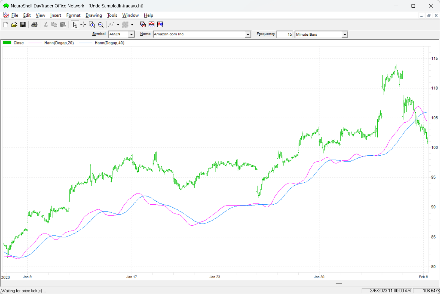
FIGURE 5: NEUROSHELL TRADER. This NeuroShell Trader chart demonstrates the undersampled intraday double moving average indicator.
Users of NeuroShell Trader can go to the Stocks & Commodities section of the NeuroShell Trader free technical support website to download a copy of this or any previous Traders’ Tips.
—Ward Systems Group, Inc.
sales@wardsystems.com
www.neuroshell.com
BACK TO LIST

The Zorro Project: April 2023
All smoothing indicators, such as the simple moving average (SMA) or lowpass filter, trade more lag for more smoothing. In this issue’s article “Just Ignore Them,” John Ehlers suggests undersampling the price curves for achieving a better compromise between smoothness and lag. We can check that out by applying a Hann filter to the original price curve and a five-fold undersampled curve.
The C code for the Hann filter, from Ehlers’ article, is:
var Hann(vars Data,int Length)
{
  var Filt = 0, Coeff = 0;
  int i;
  for(i=1; i<=Length; i++) {
    Filt += (1-cos(2*PI*i/(Length+1)))*Data[i-1];
    Coeff += 1-cos(2*PI*i/(Length+1));
  }
  return Filt/fix0(Coeff);
}
The fix0 function in the denominator has the purpose of working around division-by-zero issues. We will now apply the Hann filter to the undersampled SPY price curve:
void run()
{
  StartDate = 20220101;
  EndDate = 20221231;
  BarPeriod = 1440;

  set(PLOTNOW);
  asset("SPY");

  vars Samples = series();
  if(Init || Bar%5 == 0)
    Samples[0] = priceC(0);
  else
    Samples[0] = Samples[1];

  plot("Hann6",Hann(Samples,6),LINE,MAGENTA);
  plot("Hann12",Hann(Samples,12),LINE,BLUE);
  plot("Hann",Hann(seriesC(),12),0,DARKGREEN);
}
The resulting chart is shown in Figure 6. The blue line is the Hann filter of the undersampled curve with period 12, and magenta line with period 6. For comparison, we’ve added the Hann filter output from the original curve (green). You can see that the green line has less lag but is also less smooth.
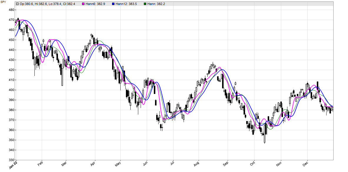
FIGURE 6: ZORRO PROJECT. This chart of the daily SPY applies a Hann filter to the original price curve and a five-fold undersampled curve. The blue line is the Hann filter of the undersampled curve with period 12, and magenta line with period 6. The Hann filter output from the original curve is shown in green for comparison. You can see that the green line has less lag but is also less smooth.
A test script for the Hann indicator and undersampling can be downloaded from the 2022 script repository on https://financial-hacker.com. The Zorro platform can be downloaded from https://zorro-project.com.
—Petra Volkova
The Zorro Project by oP group Germany
https://zorro-project.com
BACK TO LIST
Microsoft Excel: April 2023
In his article in this issue, “Just Ignore Them: Undersampling The Data As A Smoothing Technique,” John Ehlers presents an interesting approach to reducing the impact of noise in the data (high-frequency components) by way of undersampling the data and taking advantage of the resulting aliasing.
We can replicate his technique in Excel by using a two-step computation:
- Undersample the data by collecting sample values a set number of bars apart. Then propagate this value forward as the sample value for the intervening bars until the next sample bar (Figure 7).
- Compute two weighted averages of the sample values using different-length Hann weighting profiles (Figure 8).
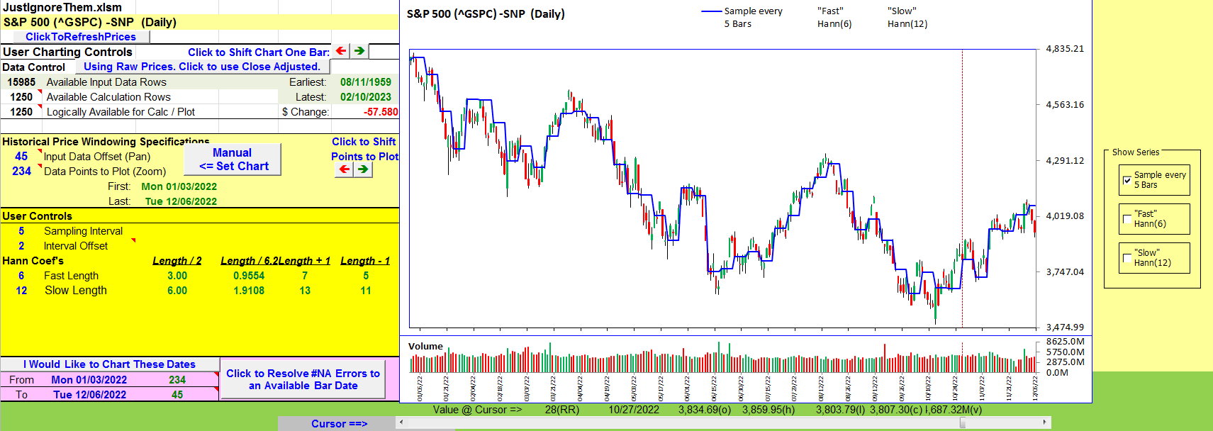
FIGURE 7: EXCEL. To replicate the smoothing technique presented in John Ehlers’ article in this issue, the first step, illustrated here, is to undersample the data by collecting sample values a set number of bars apart, then propagate this value forward as the sample value for the intervening bars until the next sample bar. Here, the closing price value is sampled every 5 bars, with the value carried forward until the next sample bar.
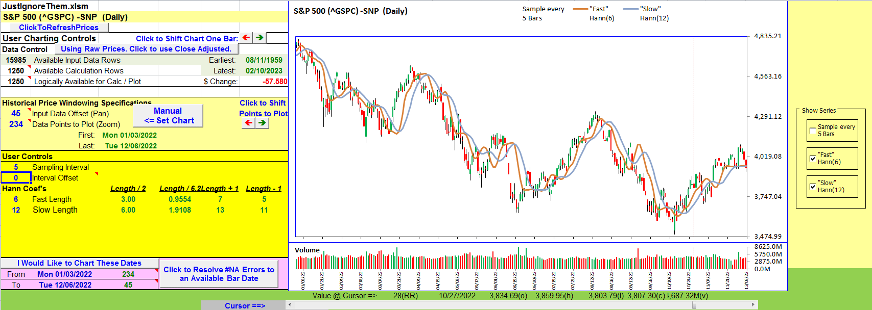
FIGURE 8: EXCEL. The next step in Excel is to compute two weighted averages of the sample values using different-length Hann weighting profiles. Here, Hann 6 and Hann 12 averages are used.
A careful observer will notice that the fast and slow Hann plots presented here do not quite match Figure 2 in Ehlers’ article in this issue. This difference really stands out in the right-most 12 or so bars. After researching this difference a bit, I determined that this is simply a case of “source data misalignment. ” It turns out that which bar we use to start the sampling and bar counting matters. Ehlers’ sampling started with a different bar.
The formulas in this spreadsheet default the starting bar of the count to be the most recent bar available (right-most bar on the chart). But the misalignment problem could be the same if my count started with the oldest bar available.
To adjust the relative starting bar, I introduced an “interval offset” in the user controls area. A non-zero “interval offset” value shifts the logical starting bar to the right. With a sampling interval of 5, valid offset values are 0 through 4. Under the covers, higher offset values logically wrap back into 0 through 4 via a modulo calculation based on the sampling interval value.
An interval offset of 3 produced a chart (Figure 9) that is a near match to Ehlers’ Figure 2. It was interesting to observe the changes of the fast and slow shapes and crossovers as I cycled through the possible interval offset values.
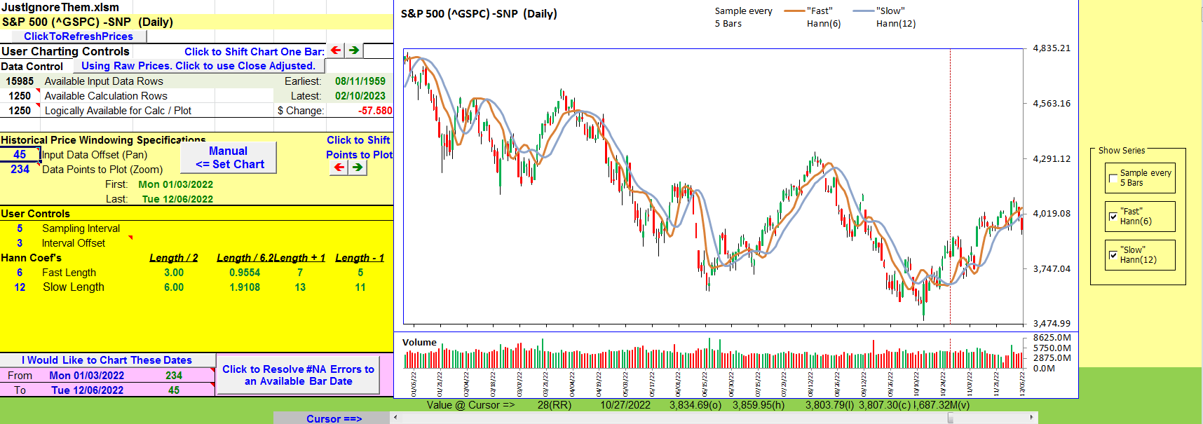
FIGURE 9: EXCEL. Here, an interval offset is chosen (of “3”) to match Figure 2 in John Ehlers’ article in this issue.
Determining the starting bar for the sampling process becomes particularly important as new data bars become available and older bars drop out of the calculation and charting window over time.
In Figure 10, I stepped 7 days forward in time without changing the interval offset. Here, the fast and slow shapes of the right-most bars look very similar to Figure 7. (Changing the interval offset to “4” restored the picture.)
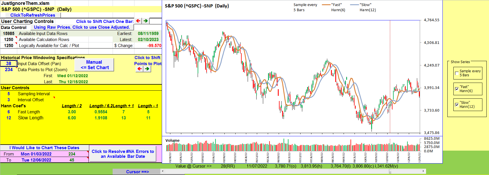
FIGURE 10: EXCEL. Seven days into the future, the fast and slow once again look similar to Figure 1 in John Ehlers’ article in this issue.
With a sampling interval of 5, the fast and slow shapes for mid-plot bars will exhibit a repeating cycle every fifth new bar. This is similar to what we observed as we cycled the interval offset value.
A possible solution would be to specify a particular bar date as an anchor for the sampling interval rather than an interval offset. And you might need to keep track of that date for each symbol you look at.
To download this spreadsheet: The spreadsheet file for this Traders’ Tip can be downloaded here. To successfully download it, follow these steps:
- Right-click on the Excel file link, then
- Select “save as” (or “save target as”) to place a copy of the spreadsheet file on your hard drive.
—Ron McAllister
Excel and VBA programmer
rpmac_xltt@sprynet.com
BACK TO LIST
Originally published in the April 2023 issue of
Technical Analysis of STOCKS & COMMODITIES magazine.
All rights reserved. © Copyright 2023, Technical Analysis, Inc.