It doesn't matter whether you analyze markets using technical or fundamental methods. If you're interested in trends and patterns, you're using time series data. You've probably illustrated trends and patterns using a chart with time on the horizontal axis and the dependent measure (price, volume and so forth) on the vertical axis. This format is simply a time series format. So whenever a time series is discussed, think of a simple bar chart.
Logic favors the idea that all elements of a single time series -- that is, the individual observations -- share defining properties. Observations in the first half of a time series should measure the same thing as in the second half. What sort of a time series might not? Consider a time series composed of a single corporation's stock price before and after a merger. A merger could be a radical change in the fundamentals of the company, and so the data would lack the homogeneity needed for all observations to share defining properties. Other, less conspicuous changes, such as shifts in industry, market, economy or political stability, can erode the necessary homogeneity. You can't compare apples and oranges in the same time series.
STATIONARITY
Stationarity is the statistical equivalent of homogeneity. Stationarity is present when variables governing a time series exert a stable influence on the data throughout the series. However, when these variables change, statistical integrity of the time series can decay.
Further, observations in the first half of the time series may not be comparable to observations in the second half. An extreme example would be if you were looking at a chart that was half the Standard & Poor's 500 stock index and half the NASDAQ Composite Index. The statistical significance of nonstationarity is important, as undetected nonstationarity can lead to costly decision errors.

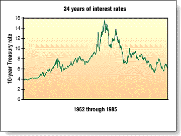
Figure 1: 10-year Treasury interest rates, 1962-85. In the second half of 1979, the slope and volatility of rates changed dramatically as rates jumped from about 9% to more than 15% within three years.
ASSESSING STATIONARITY (CHARTS)
Figure 1 illustrates 10-year Treasury interest rates from 1962 through 1985. In the second half of 1979, the slope and volatility of rates changed dramatically as rates jumped from about 9% to more than 15% within three years. The period was characterized by volatile world markets, soaring inflation and international instability.
Variables influencing interest rates had changed. Rates during the first half of the period were not governed the same way as rates in the second half were, and Figure 1 illustrates the transformation.