TRADERS’ TIPS
February 2014

For this month’s Traders’ Tips, the focus is Oscar Cagigas’s article in this issue, “The Degree Of Complexity.” Here we present the February 2014 Traders’ Tips code with possible implementations in various software.
Code for AmiBroker is already provided in Cagigas’s article. Subscribers will find that code at the Subscriber Area of our website, www.traders.com. (Click on “Article Code” from the S&C menu.) Presented here is an overview of possible implementations for other software.
Traders’ Tips code is provided to help the reader implement a selected technique from an article in this issue. The entries are contributed by various software developers or programmers for software that is capable of customization.

TRADESTATION: FEBRUARY 2014
In “The Degree Of Complexity” in this issue, author Oscar Cagigas discusses building trading systems and the impact of adding increasing complexity. He presents a simple breakout system based on the well-known Donchian channel. The author tests the strategy performance on a portfolio of 11 commodities over a period of 10 years.
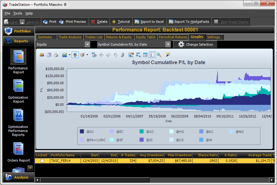
Here, we present some strategy code in EasyLanguage based on Cagigas’s basic system (two parameters) as well as the more complex four-parameter system. For this task, we can use TradeStation’s Portfolio Maestro (Figure 1) to backtest, optimize, and fully analyze the portfolio.

FIGURE 1: TRADESTATION, CUMULATIVE P/L. Using TradeStation’s Portfolio Maestro to backtest, optimize, and analyze a sample portfolio, here is a sample cumulative profit & loss (P/L) over the period 2003–2013 by security.
To download the EasyLanguage code, please visit our TradeStation and EasyLanguage support forum. The EasyLanguage code based on Cagigas’s article can be found here: https://www.tradestation.com/TASC-2014. The ELD filename is “_TASC_DonchianSystem.ELD.”
For more information about EasyLanguage in general, please see https://www.tradestation.com/EL-FAQ.
_TASC_DonchianSystem (Indicator)

{Reference: Technical Analysis of Stocks & Commodities,
Feb 2014.
Article: The Degree Of Complexity

Basic and Complex 4 parameter system

Usage Notes:
To test the 'Basic' System set the following
inputs to:

ATRVolCoef = 0
ATRStopLossMult = 0
}

inputs:
	int EntryChannelLength( 40 ),
	int ExitChannelLength( 15 ),
	int ATRLength( 20 ),
	double ATRVolCoef( .9 ),
	double ATRStopLossMult( 4 ) ;

variables:
	double UpperEntryChannel( 0 ),
	double LowerEntryChannel( 0 ),
	double UpperExitChannel( 0 ),
	double LowerExitChannel( 0 ),
	double StopATR( 0 ),
	bool EntryVolOK( false ) ;


UpperEntryChannel = Highest( High, EntryChannelLength ) ;
LowerEntryChannel = Lowest( Low, EntryChannelLength ) ;
UpperExitChannel = Highest( High, ExitChannelLength ) ;
LowerExitChannel = Lowest( Low, ExitChannelLength ) ;

StopATR = AvgTrueRange( ATRLength ) ;
EntryVolOK = AvgTrueRange( 1 ) < StopATR[1] * ATRVolCoef ;

if EntryVolOK or ATRVolCoef = 0 then
	begin
	Buy next bar at UpperEntryChannel Stop ;
	SellShort next bar at LowerEntryChannel Stop ;
	end ;

if MarketPosition = 1 then
	begin
	Sell next bar at LowerExitChannel Stop ;
	if ATRStopLossMult <> 0 then
		Sell next bar at
		EntryPrice - StopATR * ATRStopLossMult Stop ;
	end
else if MarketPosition = -1 then
	begin
	BuyToCover next bar at UpperExitChannel Stop ;
	if ATRStopLossMult <> 0 then
		BuyToCover next bar at
		EntryPrice + StopATR * ATRStopLossMult Stop ;
	end ;
This article is for informational purposes. No type of trading or investment recommendation, advice, or strategy is being made, given, or in any manner provided by TradeStation Securities or its affiliates.
—Doug McCrary
TradeStation Securities, Inc.
www.TradeStation.com
BACK TO LIST

eSIGNAL: FEBRUARY 2014
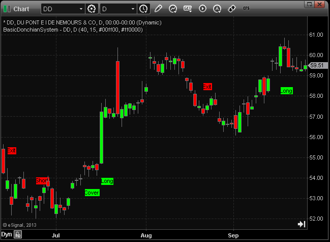
For this month’s Traders’ Tip, we’ve provided the formula BasicDonchianSystem.efs based on the formulas described in Oscar Cagigas’s article in this issue, “The Degree Of Complexity.”
The study contains formula parameters for Len1, Len2, long color, and short color, all of which may be configured through the edit chart window (right-click on “chart” and select edit chart). A sample chart is shown in Figure 2.

FIGURE 2: eSIGNAL SAMPLE CHART
To discuss this study or download a complete copy of the formula code, please visit the EFS Library Discussion Board forum under the forums link from the support menu at www.esignal.com or visit our EFS KnowledgeBase at https://www.esignal.com/support/kb/efs/. The eSignal formula script (EFS) is also available for copying & pasting below.
/*********************************
Provided By:
    Interactive Data Corporation (Copyright ?© 2013)
    All rights reserved. This sample eSignal Formula Script (EFS)
    is for educational purposes only. Interactive Data Corporation
    reserves the right to modify and overwrite this EFS file with
    each new release.

Description:
    The Degree Of Complexity by Oscar G. Cagigas

Formula Parameters:                     Default:
Len1                                    40

Len2                                    15

Long Color                              lime

Short Color                             red


Version:            1.00  12/05/2013

Notes:
    The related article is copyrighted material. If you are not a subscriber
    of Stocks & Commodities, please visit www.traders.com.

**********************************/

var fpArray = new Array();

function preMain()
{
    setStudyTitle("BasicDonchianSystem");

    setPriceStudy(true);

    var x = 0;

    fpArray[x] = new FunctionParameter("fpLen1", FunctionParameter.NUMBER);
    with(fpArray[x++])
    {
        setName("Len1");
        setLowerLimit(20);

        setUpperLimit(40);
        setDefault(40);
    }


    fpArray[x] = new FunctionParameter("fpLen2", FunctionParameter.NUMBER);
    with(fpArray[x++])
    {
        setName("Len2");
        setLowerLimit(5);

        setUpperLimit(30);
        setDefault(15);
    }


    fpArray[x] = new FunctionParameter("gLongColor", FunctionParameter.COLOR);
    with(fpArray[x++])
    {
        setName("Long Color");
        setDefault(Color.lime);
    }

    fpArray[x] = new FunctionParameter("gShortColor", FunctionParameter.COLOR);
    with(fpArray[x++])
    {
        setName("Short Color");
        setDefault(Color.red);
    }
}

var bInit = false;
var bVersion = null;

var xHHV1 = null;

var xLLV1 = null;


var xHHV2 = null;

var xLLV2 = null;


var xHigh = null;

var xLow  = null;

var xOpen = null;


function main(fpLen1,fpLen2,gLongColor,gShortColor)
{
    if (bVersion == null) bVersion = verify();
    if (bVersion == false) return;

    if (!bInit)
    {

        xHigh = high();

        xLow = low();

        xOpen = open();


        xHHV1 = hhv(fpLen1, xHigh);

        xLLV1 = llv(fpLen1, xLow);


        xHHV2 = hhv(fpLen2, xHigh);

        xLLV2 = llv(fpLen2, xLow);


        bInit = true;
    }


    var nBuyStop   = xHHV1.getValue(-1);

    var nSellStop  = xLLV2.getValue(-1);

    var nShortStop = xLLV1.getValue(-1);

    var nCoverStop = xHHV2.getValue(-1);


    var nHigh = xHigh.getValue(0);

    var nLow  = xLow.getValue(0);

    var nOpen = xOpen.getValue(0);


    if (nBuyStop == null || nSellStop == null || nShortStop == null || nCoverStop == null || nHigh == null || nLow == null || nOpen == null)

        return;


    nPrice=null;


    if (getCurrentBarIndex() != 0)
    {

            // Entry Strategy
            if (!Strategy.isInTrade())
            {
               //LONG ENTRY

                    if (nHigh > nBuyStop)

                    {

                       Strategy.doLong("Enter Long", Strategy.CLOSE, Strategy.THISBAR);

                       drawTextRelative(0, BelowBar2, "Long", Color.black, gLongColor, Text.PRESET, null, null);
                    }

                else

                {

                    //SHORT ENTRY

                    if (nLow < nShortStop)
                    {

                       Strategy.doShort("Enter Short", Strategy.CLOSE, Strategy.THISBAR);

                       drawTextRelative(0, AboveBar2, "Short", Color.black, gShortColor, Text.PRESET, null, null);
                    }

                }
            }


            // Exit Strategy
            if (Strategy.isInTrade())
            {

                //EXIT

                if ((nLow < nSellStop) && Strategy.isLong())
                        {

                           Strategy.doSell("Exit", Strategy.CLOSE, Strategy.THISBAR);

                           drawTextRelative(0, AboveBar2, "Exit", Color.black, gShortColor, Text.PRESET, null, null);
                        }

                else

                    {

                        //COVER

                        if ((nHigh > nCoverStop) && Strategy.isShort())
                        {

                           Strategy.doCover("Cover", Strategy.CLOSE, Strategy.THISBAR);

                           drawTextRelative(0, BelowBar2, "Cover", Color.black, gLongColor, Text.PRESET, null, null);
                        }

                }

            }
        }


    return;
}

function verify()
{
    var b = false;
    if (getBuildNumber() < 779)
    {
        drawTextAbsolute(5, 35, "This study requires version 8.0 or later.",
            Color.white, Color.blue, Text.RELATIVETOBOTTOM|Text.RELATIVETOLEFT|Text.BOLD|Text.LEFT,
            null, 13, "error");
        drawTextAbsolute(5, 20, "Click HERE to upgrade.@URL=https://www.esignal.com/download/default.asp",
            Color.white, Color.blue, Text.RELATIVETOBOTTOM|Text.RELATIVETOLEFT|Text.BOLD|Text.LEFT,
            null, 13, "upgrade");
        return b;
    }
    else
    {
        b = true;
    }

    return b;
}
—Jason Keck
eSignal, an Interactive Data company
800 779-6555, www.eSignal.com
BACK TO LIST

THINKORSWIM: FEBRUARY 2014
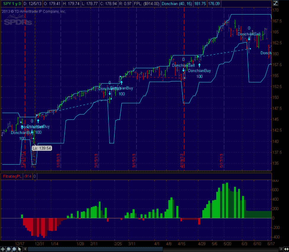
In “The Degree Of Complexity” in this issue, author Oscar Cagigas describes how to build a trading system with a low level of complexity. For thinkorswim users, we have recreated this strategy in our proprietary scripting language, thinkScript. To get the strategy, simply go to: https://tos.mx/s7sg5S
You can adjust the parameters within the edit studies window to fine-tune your variables. A sample chart implementation is shown in Figure 3.

FIGURE 3: THINKORSWIM
Alternatively, you can manually load the strategy code by following these steps:
- From TOS charts, select Studies → Edit studies
- Select the strategy tab in the upper left-hand corner
- Select “new” in the lower left-hand corner
- Name the strategy (for example, “DonchianStrategy”)
- Click in the script editor window, remove “addOrder(OrderType.BUY_AUTO, no);” and paste in the following code:
input length1 = 40;
input length2 = 15;

def buystop = Highest(high, length1)[1];
def sellstop = Lowest(low, length2)[1];
def shortstop = Lowest(low, length1)[1];
def coverstop = Highest(high, length2)[1];

def buy = high > buystop;
def short = low < shortstop;
def sell = low < sellstop;
def cover = high > coverstop;

def position = {default none, long, short};
position = if (buy or (position[1] == position.long and !sell)) then position.long else if (short or (position[1] == position.short and !cover)) then position.short else position.none;

plot BandUp = if position[1] == position.short then coverstop else buystop;
plot BandDown = if position[1] == position.long then sellstop else shortstop;
BandUp.SetDefaultColor(GetColor(1));
BandDown.SetDefaultColor(GetColor(1));

AddOrder(OrderType.BUY_AUTO, buy, tickColor = GetColor(1), arrowColor = GetColor(1), name = "DonchianBuy");
AddOrder(OrderType.SELL_AUTO, short, tickColor = GetColor(1), arrowColor = GetColor(1), name = "DonchianShort");
AddOrder(OrderType.SELL_TO_CLOSE, sell, tickColor = GetColor(1), arrowColor = GetColor(1), name = "DonchianSell");
AddOrder(OrderType.BUY_TO_CLOSE, cover, tickColor = GetColor(1), arrowColor = GetColor(1), name = "DonchianCover");
—thinkorswim
A division of TD Ameritrade, Inc.
www.thinkorswim.com
BACK TO LIST

METASTOCK: FEBRUARY 2014
Oscar Cagigas’s article in this issue, “The Degree Of Complexity,” discusses how simpler systems can perform better than more complex ones. Formulas for MetaStock to implement Cagigas’s basic Donchian channel system are provided here.
Buy Order:

Len1:= OPT1;
Len2:= OPT2;
el:= h > ref(hhv(H,len1),-1);
es:= L < ref(llv(L,len1),-1);
xl:= L < ref(llv(L,len2),-1);
xs:= h > ref(hhv(H,len2),-1);
trade:= if(el, 1, if(es, -1,
if((prev=1 and xl) or (prev=-1 and xs), 0, prev)));
trade=1 and ref(trade<>1, -1)

Sell Order:

Len1:= OPT1;
Len2:= OPT2;
el:= h > ref(hhv(H,len1),-1);
es:= L < ref(llv(L,len1),-1);
xl:= L < ref(llv(L,len2),-1);
xs:= h > ref(hhv(H,len2),-1);
trade:= if(el, 1, if(es, -1,
if((prev=1 and xl) or (prev=-1 and xs), 0, prev)));
trade=0 and ref(trade=1, -1)

Sell Short Order:

Len1:= OPT1;
Len2:= OPT2;
el:= h > ref(hhv(H,len1),-1);
es:= L < ref(llv(L,len1),-1);
xl:= L < ref(llv(L,len2),-1);
xs:= h > ref(hhv(H,len2),-1);
trade:= if(el, 1, if(es, -1,
if((prev=1 and xl) or (prev=-1 and xs), 0, prev)));
trade=-1 and ref(trade<>-1, -1)

Buy to Cover Order:

Len1:= OPT1;
Len2:= OPT2;
el:= h > ref(hhv(H,len1),-1);
es:= L < ref(llv(L,len1),-1);
xl:= L < ref(llv(L,len2),-1);
xs:= h > ref(hhv(H,len2),-1);
trade:= if(el, 1, if(es, -1,
if((prev=1 and xl) or (prev=-1 and xs), 0, prev)));
trade=0 and ref(trade=-1, -1)

Optimizations:

OPT1:
Description:  long term
Minimum: 20
Maximum: 40
Step : 5

OPT2:
Description:  short term
Minimum: 5
Maximum: 20
Step : 5
—William Golson
MetaStock Technical Support
www.metastock.com
BACK TO LIST

NEUROSHELL TRADER: FEBRUARY 2014
The Donchian channel trading system described by Oscar Cagigas in his article in this issue, “The Degree Of Complexity,” can be easily implemented with a few of NeuroShell Trader’s 800+ indicators. Simply select “New trading strategy” from the Insert menu and enter the following in the appropriate locations of the NeuroShell trading strategy wizard:
Generate a buy long STOP order if all of the following are true:
    	High Channel Breakout(High,40)
	Stop Price: Lag(Max(High,40),1)
Generate a sell short STOP order if all of the following are true:
    	Low Channel Breakout(Low,15)
	Stop Price: Lag(Min(Low,15),1)
If you have NeuroShell Trader Professional, you can also choose whether the parameters should be optimized. After backtesting the trading strategy, use the “Detailed analysis” button to view the backtest and trade-by-trade statistics for the strategy.
Users of NeuroShell Trader can go to the STOCKS & COMMODITIES section of the NeuroShell Trader free technical support website to download a copy of this or any previous Traders’ Tips.
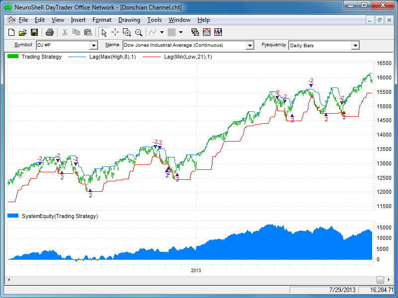
A sample chart is shown in Figure 4.

FIGURE 4: NEUROSHELL TRADER. This NeuroShell Trader chart displays the out-of-sample Donchian channel trading after optimizing on prior data.
—Marge Sherald, Ward Systems Group, Inc.
301 662-7950, sales@wardsystems.com
www.neuroshell.com
BACK TO LIST

AIQ: FEBRUARY 2014
This Traders’ Tip is based on “The Degree Of Complexity” by Oscar Cagigas in this issue.
The five Donchian breakout systems described by Cagigas in his article are coded using the following rules:
| System |
Entry rule |
Exit rule |
Entry price formula |
Exit price formula |
| 2 Param-Long |
Buy2P |
ExitBuy2P |
Buy2Ppr |
ExitBuy2Ppr |
| 2 Param-Short |
Sell2P |
ExitSell2P |
Sell2Ppr |
ExitSell2Ppr |
| 4 Param-Long |
Buy4P |
ExitBuy4P |
Buy4Ppr |
ExitBuy4Ppr |
| 4 Param-Short |
Sell4P |
ExitSell4P |
ell4Ppr |
ExitSell4Ppr |
| 6 Param-Long |
Buy6P |
ExitBuy6P |
Buy6Ppr |
ExitBuy6Ppr |
| 6 Param-Short |
Sell6P |
ExitSell6P |
Sell6Ppr |
ExitSell6Ppr |
| 8 Param-Long |
Buy8P |
ExitBuy8P |
Buy8Ppr |
ExitBuy8Ppr |
| 8 Param-Short |
Sell8P |
ExitSell8P |
Sell8Ppr |
ExitSell8Ppr |
| 9 Param-Long |
Buy9P |
ExitBuy9P |
Buy9Ppr |
ExitBuy9Ppr |
| 9 Param-Short |
Sell9P |
ExitSell9P |
Sell9Ppr |
ExitSell9Ppr |
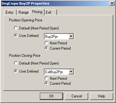
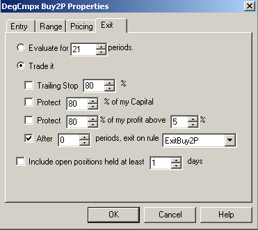
The EDS code file has the backtests already set up for all of these long and short rules. In Figure 5, I show a typical setup for the pricing. In Figure 6, I show a typical setup for the exit rule.

FIGURE 5: AIQ. Here is a typical setup for the pricing portion of the backtests.

FIGURE 6: AIQ. Here is a typical setup for the exit portion of the backtests.
The AIQ code and EDS file can be downloaded from www.TradersEdgeSystems.com/traderstips.htm, and is also shown below.
!THE DEGREE OF COMPLEXITY

!Author: Oscar G. Cagigas, TASC Feb 2014

!Coded by Richard Denning 12/7/13

!www.TradersEdgeSystems.com


! CODING ABBREVIATIONS:

C	is [close].

H 	is [high].

L 	is [low].

O	is [open].

PEP 	is {position entry price}.

PD    	is {position days}.


! PARAMETERS:

donLen1	is 40.

donLen2	is 15.

atrLen	is 20.

atrMult	is 1.0.

atrStop 	is 4.0.

maLen1 	is 10.

maLen2 	is 100.

rsiLen	is 14.

rsiUpper 	is 70.

rsiLower 	is 30.

atrMult2	is 0.6.

minMov	is 0.01.

!------------------------------------------------------------------

! AVERAGE TRUE RANGE (AS DEFINED BY WELLS WILDER)

WWE	is 2*(atrLen-1).

TR 	is Max(H - L,max(abs(valresult(C,1) - L),abs(valresult(C,1)- H))).

ATR	is expAvg(TR,WWE).

ATR1	is valresult(ATR,1).

!------------------------------------------------------------------

!! RSI WILDER

!To convert Wilder Averaging to Exponential Averaging use this formula:

!ExponentialPeriods = 2 * WilderPeriod - 1.

U 	is C-valresult(C,1).

D 	is valresult(C,1)-C.

eLen	is 2 * rsiLen - 1.

AvgU 	is ExpAvg(iff(U>0,U,0),eLen).

AvgD 	is ExpAvg(iff(D>=0,D,0),eLen).

rsi 	is 100-(100/(1+(AvgU/AvgD))).

!----------------------------------------------------------------

!BASIC SYSTEM 2P (2 parameters):

HHdL1 is  highresult(H,donLen1,1).

HHdL2 is  highresult(H,donLen2,1).

LLdL1 is lowresult(L,donLen1,1).

LLdL2 is lowresult(L,donLen2,1).

Buy2P if H > HHdL1.

ExitBuy2P if  L < LLdL2.

Sell2P if L < LLdL1.

ExitSell2P if H > HHdL2.

Buy2Ppr is max(O,HHdL1 + minMov).

ExitBuy2Ppr is iff(ExitBuy2P,min(O,LLdL2 - minMov),C).

Sell2Ppr is min(O,LLdL1 - minMov).

ExitSell2Ppr is max(O,HHdL2 + minMov).

!-----------------------------------------------------------------

!FOUR PARAMETER SYSTEM 4P:

Buy4P if H > HHdL1 and valrule(TR < atrMult*ATR,1).

EB4P1 if L < LLdL2.

EB4Pval is PEP - atrStop*valresult(ATR,PD).

EB4P2 if L < valresult(EB4Pval,1).

ExitBuy4P if EB4P1 or EB4P2.

Sell4P if L < LLdL1 and valrule(TR < atrMult*ATR,1).

ES4Pval is PEP + atrStop*valresult(ATR,PD) .

ES4P1 if H > HHdL2.

ES4P2 if H > valresult(ES4Pval,1).

ExitSell4P if ES4P1 or ES4P2.

Buy4Ppr is max(O,HHdL1 + minMov).

ExitBuy4Ppr is iff(EB4P1,min(O,LLdL2 - minMov),

	iff(EB4P2,min(O,valresult(EB4Pval - minMov,1)),-99)).

Sell4Ppr is min(O,LLdL1 - minMov).

ExitSell4Ppr is iff(ES4P1,max(O,HHdL2 + minMov),

	iff(ES4P2,max(O,valresult(ES4Pval + minMov,1)),-99)).

!----------------------------------------------------------------

!SIX PARAMETER SYSTEM 6P:

SMA1 is simpleavg(C,maLen1).

SMA2 is simpleavg(C,maLen2).

Buy6P if H > HHdL1 and valrule(TR < atrMult*ATR,1)

	and valrule(SMA1 > SMA2,1).

EB6P1 if L < LLdL2.

EB6Pval is PEP - atrStop*valresult(ATR,PD).

EB6P2 if L < valresult(EB6Pval,1).

ExitBuy6P if EB6P1 or EB6P2.

Sell6P if L < LLdL1 and valrule(TR < atrMult*ATR,1)

	and valrule(SMA1 < SMA2,1).

ES6Pval is PEP + atrStop*valresult(ATR,PD) .

ES6P1 if H > HHdL2.

ES6P2 if H > valresult(ES6Pval,1).

ExitSell6P if ES6P1 or ES6P2.

Buy6Ppr is max(O,HHdL1 + minMov).

ExitBuy6Ppr is iff(EB6P1,min(O,LLdL2 - minMov),

	iff(EB6P2,min(O,valresult(EB6Pval - minMov,1)),-99)).

Sell6Ppr is min(O,LLdL1 - minMov).

ExitSell6Ppr is iff(ES6P1,max(O,HHdL2 + minMov),

	iff(ES6P2,max(O,valresult(ES6Pval + minMov,1)),-99)).

!---------------------------------------------------------------

!EIGHT PARAMETER SYSTEM 8P:

Buy8P if H > HHdL1 and valrule(TR < atrMult*ATR,1)

	and valrule(SMA1 > SMA2,1) and valrule(RSI >= rsiUpper,1).

EB8P1 if L < LLdL2.

EB8Pval is PEP - atrStop*valresult(ATR,PD).

EB8P2 if L < valresult(EB8Pval,1).

ExitBuy8P if EB8P1 or EB8P2.

Sell8P if L < LLdL1 and valrule(TR < atrMult*ATR,1)

	and valrule(SMA1 < SMA2,1) and valrule(RSI <= rsiLower,1).

ES8Pval is PEP + atrStop*valresult(ATR,PD) .

ES8P1 if H > HHdL2.

ES8P2 if H > valresult(ES8Pval,1).

ExitSell8P if ES8P1 or ES8P2.

Buy8Ppr is max(O,HHdL1 + minMov).

ExitBuy8Ppr is iff(EB8P1,min(O,LLdL2 - minMov),

	iff(EB8P2,min(O,valresult(EB8Pval - minMov,1)),-99)).

Sell8Ppr is min(O,LLdL1 - minMov).

ExitSell8Ppr is iff(ES8P1,max(O,HHdL2 + minMov),

	iff(ES8P2,max(O,valresult(ES8Pval + minMov,1)),-99)).

!----------------------------------------------------------------

!NINE PARAMETER SYSTEM 9P:

Buy9P if H > HHdL1 and valrule(TR < atrMult*ATR,1)

	and valrule(SMA1 > SMA2,1) and valrule(RSI >= rsiUpper,1)

	and valrule(TR > atrmult2*ATR,1) .

EB9P1 if L < LLdL2.

EB9Pval is PEP - atrStop*valresult(ATR,PD).

EB9P2 if L < valresult(EB9Pval,1).

ExitBuy9P if EB9P1 or EB9P2.

Sell9P if L < LLdL1 and valrule(TR < atrMult*ATR,1)

	and valrule(SMA1 < SMA2,1) and valrule(RSI <= rsiLower,1)

	and valrule(TR > atrmult2*ATR,1) .

ES9Pval is PEP + atrStop*valresult(ATR,PD) .

ES9P1 if H > HHdL2.

ES9P2 if H > valresult(ES9Pval,1).

ExitSell9P if ES9P1 or ES9P2.

Buy9Ppr is max(O,HHdL1 + minMov).

ExitBuy9Ppr is iff(EB9P1,min(O,LLdL2 - minMov),

	iff(EB9P2,min(O,valresult(EB9Pval - minMov,1)),-99)).

Sell9Ppr is min(O,LLdL1 - minMov).

ExitSell9Ppr is iff(ES9P1,max(O,HHdL2 + minMov),

	iff(ES9P2,max(O,valresult(ES9Pval + minMov,1)),-99)).

!----------------------------------------------------------------
—Richard Denning
info@TradersEdgeSystems.com
for AIQ Systems
BACK TO LIST

TRADERSSTUDIO: FEBRUARY 2014
The TradersStudio code for Oscar Cagigas’s systems presented in his article in this issue, “The Degree Of Complexity,” can be found at:
The following code files are contained in the download:
- System: DON2P – Basic Donchian system with two parameters
- System: DON4P – Donchian system with four parameters
- System: DON6P – Donchian system with six parameters
- System: DON8P – Donchian system with eight parameters
- System: DON9P – Donchian system with nine parameters
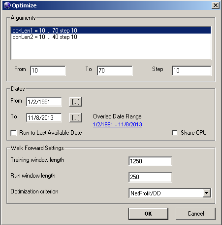
The in-sample and out-of-sample tests discussed by Cagigas could be run using TradersStudio’s built-in walk-forward processor. Figure 7 shows the typical setup in TradersStudio to run a walk-forward optimization for the DON2P system.

FIGURE 7: TRADERSSTUDIO. Here is a typical setup for running a walk-forward optimization in TradersStudio.
—Richard Denning
info@TradersEdgeSystems.com
for TradersStudio
BACK TO LIST

WEALTH-LAB: FEBRUARY 2014
The asymmetrical Donchian channel breakout system discussed in Oscar Cagigas’s article in this issue (“The Degree Of Complexity”) for model purposes is already built into Wealth-Lab. Thus, we don’t need to provide code this time around. The feature is called Channel Breakout VT and can be found under the breakouts folder in the “open strategy” dialog (Ctrl-O). Traders can control the channel periods interactively through strategy parameter sliders.
—Eugene, Wealth-Lab team
MS123, LLC
www.wealth-lab.com
BACK TO LIST

NINJATRADER: FEBRUARY 2014
The Donchian trading system, as discussed by Oscar Cagigas in his article in this issue, “The Degree Of Complexity,” has been implemented as a strategy available for download at www.ninjatrader.com/SC/February2014SC.zip.
Once it has been downloaded, from within the NinjaTrader Control Center window, select the menu File → Utilities → Import NinjaScript and select the downloaded file. This file is for NinjaTrader version 7 or greater.
You can review the strategy source code by selecting the menu Tools → Edit NinjaScript → Strategy from within the NinjaTrader Control Center window and selecting the DonchianTradingSystem file.
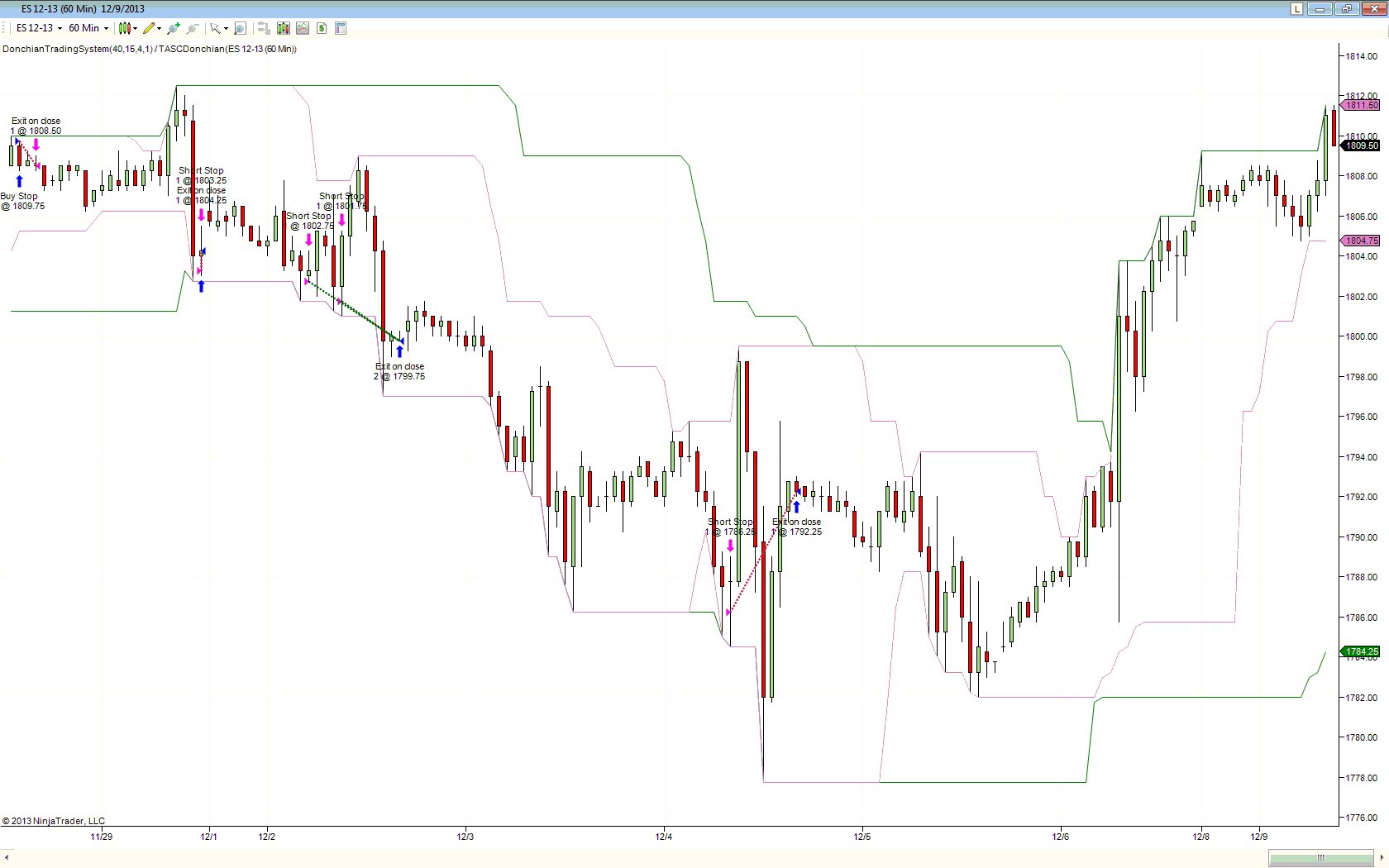
A sample chart implementing the strategy is shown in Figure 8.

FIGURE 8: NINJATRADER. This screenshot shows the Donchian trading system applied to a 60-minute chart of the emini S&P 500. The lines represent the longer Donchian channel and slower Donchian channel optimized at 40 and 15, respectively.
—Raymond Deux & Cal Hueber
NinjaTrader, LLC
www.ninjatrader.com
BACK TO LIST

UPDATA: FEBRUARY 2014
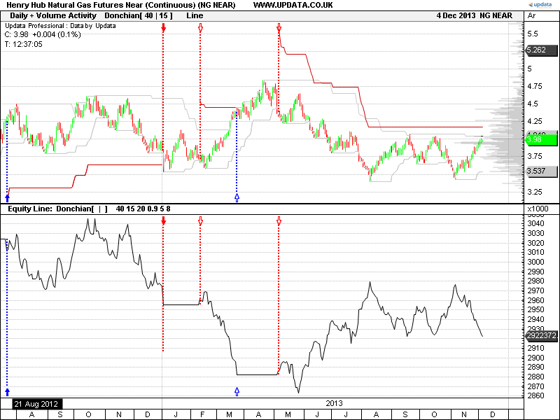
In “The Degree Of Complexity” in this issue, author Oscar Cagigas develops systems with increasingly larger numbers of factors to show the effect of backtested performance dropoff between in- and out-of-sample data. The example given in Figure 9 is of a Donchian breakout system with a volatility filter and a trailing stop exit that are both based on ATR.

FIGURE 9: UPDATA. This chart shows the Donchian ATR filter system as applied to NYMEX-listed natural gas futures in daily resolution.
The Updata code for this article is in the Updata Library and may be downloaded by clicking the custom menu and system library. Those who cannot access the library due to a firewall may paste the code below into the Updata custom editor and save it.
PARAMETER "Donchian Upper" #DONCHIANPeriodHigh=40
PARAMETER "Donchian Lower" #DONCHIANPeriodLow=15
PARAMETER "ATR Volatility Period" #ATRPeriodVol=20
PARAMETER "ATR Mult. 1" @K1=0.9
PARAMETER "ATR Stop Period" #ATRPeriodStop=5
PARAMETER "ATR Mult. 2" @K2=0.8
@ATRStopLong=0
@ATRStopShort=0
@DonchianUpper=0
@DonchianLower=0
DISPLAYSTYLE 4LINES
INDICATORTYPE TOOL
PLOTSTYLE LINE RGB(200,200,200)
PLOTSTYLE2 LINE RGB(200,200,200)
PLOTSTYLE3 LINE RGB(200,0,0)
PLOTSTYLE4 LINE RGB(200,0,0)

NAME "Donchian[" #DONCHIANPeriodHigh "|" #DONCHIANPeriodLow "]" ""
FOR #CURDATE=#DONCHIANPeriodHigh TO #LASTDATE
   @DonchianUpper=PHIGH(HIGH(1),#DONCHIANPeriodHigh)
   @DonchianLower=PLOW(LOW(1),#DONCHIANPeriodLow)
   'STOP EXIT
   IF ORDERISOPEN=1 AND LOW<@ATRStopLong
      SELL @ATRStopLong
   ELSEIF ORDERISOPEN=-1 AND HIGH>@ATRStopShort
      COVER @ATRStopShort
   ENDIF
   'DONCHIAN ENTRIES WITH ATR FILTER
   IF HIGH>@DonchianUpper AND ATR(1)<@K1*ATR(#ATRPeriodVol) AND ORDERISOPEN=0
      BUY CLOSE
      @ATRStopLong=CLOSE-@K2*ATR(#ATRPeriodStop)
   ELSEIF LOW<@DonchianLower AND ATR(1)<@K1*ATR(#ATRPeriodVol) AND ORDERISOPEN=0
      SHORT CLOSE
      @ATRStopShort=CLOSE+@K2*ATR(#ATRPeriodStop)
   ENDIF
   'TRAILING STOP
   IF ORDERISOPEN=1
      @ATRStopLong=MAX(CLOSE-@K2*ATR(#ATRPeriodStop),@ATRStopLong)
      @PLOT3=@ATRStopLong
      @PLOT4=-10000
   ELSEIF ORDERISOPEN=-1
      @ATRStopShort=MIN(CLOSE+@K2*ATR(#ATRPeriodStop),@ATRStopShort)
      @PLOT3=-10000
      @PLOT4=@ATRStopShort
   ELSE
      @PLOT3=-10000
      @PLOT4=-10000
   ENDIF
   @PLOT=@DonchianUpper
   @PLOT2=@DonchianLower
NEXT
—Updata support team
support@updata.co.uk
www.updata.co.uk
BACK TO LIST

TRADING BLOX: FEBRUARY 2014
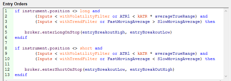
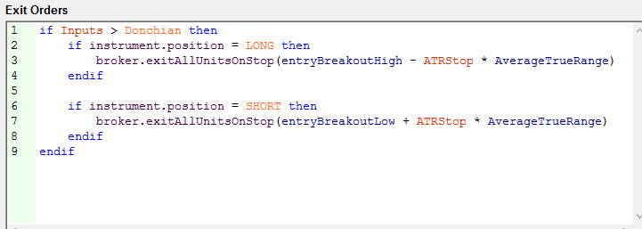
In “The Degree Of Complexity” in this issue, author Oscar Cagigas presents a Donchian breakout system with multiple sets of rules and filters. We are providing code for Trading Blox that includes the Donchian system rules (Figures 10 & 11) plus the ATR stop, volatility filter, and trend filter.

FIGURE 10: TRADING BLOX, ENTRY RULES. Here are the entry rules for the Donchian system based on Oscar Cagigas’s article in this issue.

FIGURE 11: TRADING BLOX, EXIT RULES. Here are the exit rules.
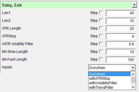
The inputs parameter (Figure 12) allows each rule or filter to be selected, inclusive of the previous one, as in Cagigas’s article.

FIGURE 12: TRADING BLOX, RULE SELECTOR. The inputs parameter allows each rule or filter to be selected, inclusive of the previous one, as in Cagigas’s article.
—Trading Blox
tradingblox.com
BACK TO LIST
MICROSOFT EXCEL: FEBRUARY 2014
Oscar Cagigas’s article in this issue, “The Degree Of Complexity,” investigates the beneficial and detrimental aspects of increasing the complexity of a trading system model in the quest to improve system performance through backtesting. Cagigas then measures the performance of the improved system model at each step by checking the results of the model on out-of-sample data.
The spreadsheet I am providing here demonstrates a version of his basic, two-parameter Donchian system that is the starting point for Cagigas’s exploration of system complexity.
Using the built-in Excel capability for data tables (Figure 13), the spreadsheet I am providing incorporates a very simple modeling capability that cycles through Len1 and Len2 values using the low, high, and step size values for each, as found in the sidebar to Cagigas’s article presenting AmiBroker code.

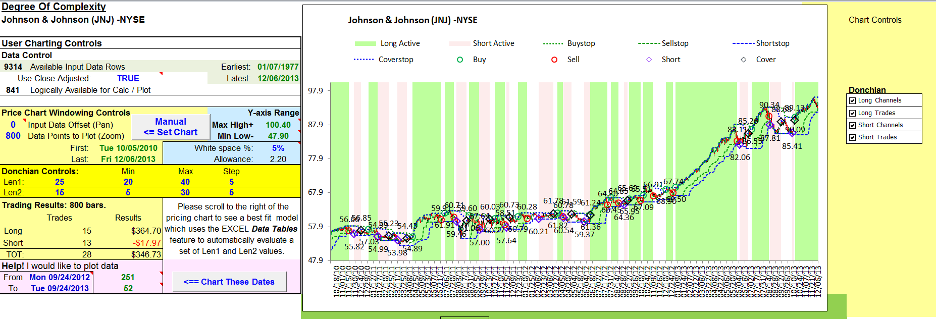
FIGURE 13: EXCEL, DONCHIAN TRADING SYSTEM. This sample chart shows Johnson & Johnson in the simple Donchian system described in Oscar Cagigas’s article in this issue, “The Degree Of Complexity.”
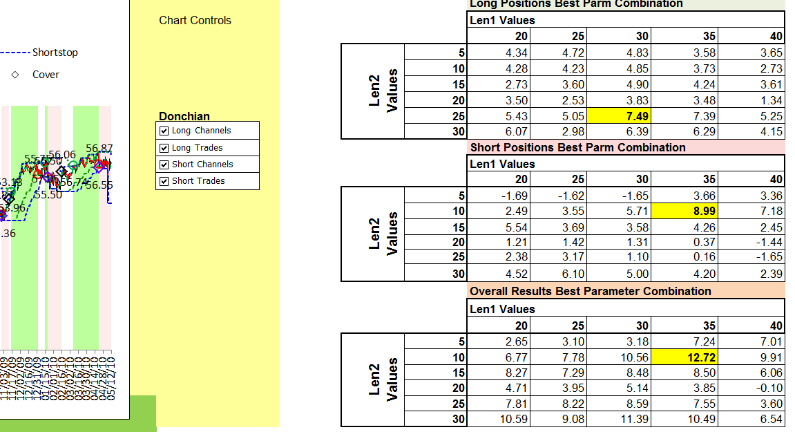
You can perform a simple backtest by specifying an offset of something like 900 and using a “points to plot” value of 800. Then click the manual set chart button and wait for things to settle. When the flickering stops, scroll to the right of the pricing chart to see the simulation results (Figure 14).

FIGURE 14: EXCEL, BEST-FIT USING OFFSET OF 900. Here is the best-fit backtest model at an offset of 900 using the built-in capability for Excel data tables.
Capture the best-fit Len1 and Len2 values from the appropriate data table and enter them in cells B16 and B17, respectively.
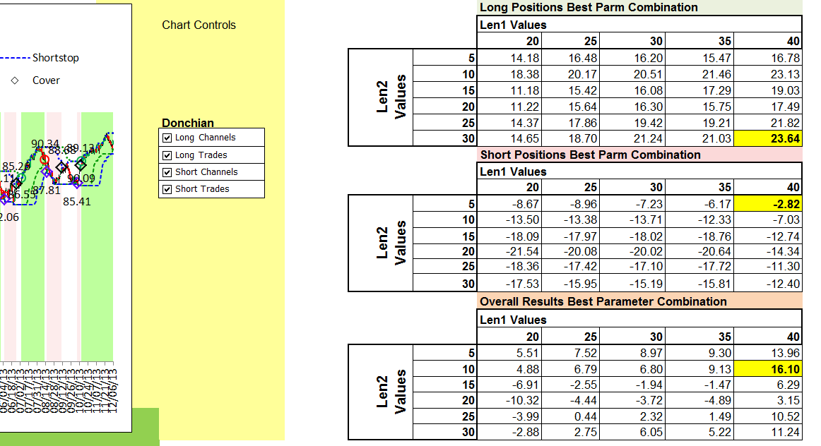
Out-of-sample testing may be simulated by setting the offset to zero, leaving the points to plot at 800.
Once again, click the manual set chart button and wait for things to settle. When the flickering stops, scroll to the right of the pricing chart to see just how much things have changed (Figure 15).

FIGURE 15: EXCEL, BEST-FIT USING OFFSET OF ZERO. Here is the best-fit “out-of-sample” using an offset of zero.
The spreadsheet file for this Traders’ Tip can be downloaded here. To successfully download it, follow these steps:
- Right-click on the Excel file link, then
- Select “save as” to place a copy of the spreadsheet file on your hard drive.
—Ron McAllister, Excel and VBA programmer
rpmac_xltt@sprynet.com
BACK TO LIST
Originally published in the February 2014 issue of
Technical Analysis of Stocks & Commodities magazine.
All rights reserved. © Copyright 2013, Technical Analysis, Inc.


