TRADERS’ TIPS
March 2010
Here is this month’s selection of Traders’ Tips, contributed by various developers of technical analysis software to help readers more easily implement some of the strategies presented in this and other issues.
Other code appearing in articles in this issue is posted in the Subscriber Area of our website at https://technical.traders.com/sub/sublogin.asp. Login requires your last name and subscription number (from mailing label). Once logged in, scroll down to beneath the “Optimized trading systems” area until you see “Code from articles.” From there, code can be copied and pasted into the appropriate technical analysis program so that no retyping of code is required for subscribers.
You can copy these formulas and programs for easy use in your spreadsheet or analysis software. Simply “select” the desired text by highlighting as you would in any word processing program, then use your standard key command for copy or choose “copy” from the browser menu. The copied text can then be “pasted” into any open spreadsheet or other software by selecting an insertion point and executing a paste command. By toggling back and forth between an application window and the open web page, data can be transferred with ease.
This month’s tips include formulas and programs for:
- TRADESTATION: EMPIRICAL MODE DECOMPOSITION
- eSIGNAL: EMPIRICAL MODE DECOMPOSITION
- METASTOCK: EMPIRICAL MODE DECOMPOSITION
- WEALTH-LAB: EMPIRICAL MODE DECOMPOSITION
- AMIBROKER: EMPIRICAL MODE DECOMPOSITION
- WORDEN BROTHERS STOCKFINDER: EMPIRICAL MODE DECOMPOSITION
- NEUROSHELL TRADER: EMPIRICAL MODE DECOMPOSITION
- AIQ: FLAT-BASE BREAKOUT SYSTEM
- TRADERSSTUDIO: EMPIRICAL MODE DECOMPOSITION
- TRADINGSOLUTIONS: EMPIRICAL MODE DECOMPOSITION
- TRADECISION: EMPIRICAL MODE DECOMPOSITION
- NINJATRADER: EMPIRICAL MODE DECOMPOSITION
- NEOTICKER: EMPIRICAL MODE DECOMPOSITION
- WAVE59: EMPIRICAL MODE DECOMPOSITION
- VT TRADER: EMPIRICAL MODE DECOMPOSITION
- EASYLANGUAGE: EMPIRICAL MODE DECOMPOSITION — ARTICLE CODE
![]() TRADESTATION: EMPIRICAL MODE DECOMPOSITION
TRADESTATION: EMPIRICAL MODE DECOMPOSITION
In their article in this issue, “Empirical Mode Decomposition,” authors John Ehlers and Ric Way suggest using methods based on bandpass filtering to distinguish trending from cycling markets. The article’s trading suggestions were used to create the EmpiricalMode strategy given here for TradeStation. If the strategy determines that the market is in trending mode, then the strategy is allowed to trade with the trend — either long, in uptrends, or short, in downtrends. If the indicator determines that the market is in cycling mode, then the strategy allows trading cycle extremes, using Bollinger bands to trigger entries.
To download the adapted EasyLanguage code, go to the TradeStation and EasyLanguage support forum (https://www.tradestation.com/Discussions/forum.aspx?Forum_ID=213). Search for the file “EmpiricalMode.eld.”
A sample chart is shown in Figure 1.
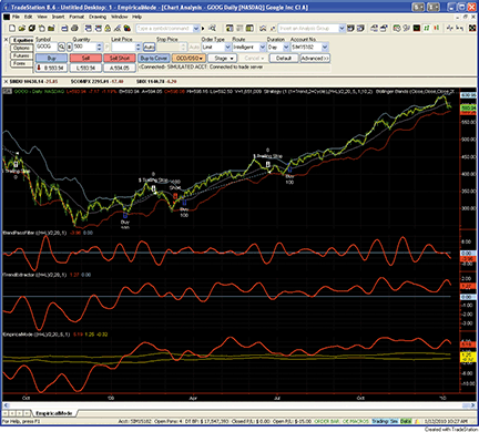
Figure 1: TRADESTATION, Empirical Mode Decomposition. A daily chart of Google, Inc. (GOOG), shows the empirical mode decomposition studies presented by John Ehlers and Ric Way in their article in this issue. The upper subgraph displays daily price bars and strategy trades based on the ModeTrader strategy. Subgraph 2 displays the band-pass filter indicator. Subgraph 3 shows the TrendExtraction indicator. Subgraph 4 shows a plot of the EmpiricalMode indicator.
This article is for informational purposes. No type of trading or investment recommendation, advice, or strategy is being made, given, or in any manner provided by TradeStation Securities or its affiliates.
Indicator:  BandPassFilter
inputs:
	Price( 0.5 * ( High + Low ) ),
	Period( 20 ),
	Delta1( 0.1 ) ;

variables:
	Beta1( 0 ),
	Gamma1( 0 ),
	Alpha( 0 ),
	HalfAlphaDiff( 0 ),
	Beta1OnePlusAlpha( 0 ),
	BP( 0 ) ;

Beta1 = Cosine( 360 / Period ) ;
Gamma1 = 1 / Cosine( 720 * Delta1 / Period ) ;
Alpha = Gamma1 - SquareRoot( Square( Gamma1 ) - 1 ) ;
HalfAlphaDiff = 0.5 * ( 1 - Alpha ) ;
Beta1OnePlusAlpha = Beta1 * ( 1 + Alpha ) ;
BP = HalfAlphaDiff * ( Price - Price[2] ) +
 Beta1OnePlusAlpha * BP[1] - Alpha * BP[2] ;

Plot1( BP, "BandPass" ) ;
Plot2( 0, "Zero" ) ;

Indicator:  TrendExtractor
inputs:
	Price( 0.5 * ( High + Low ) ),
	Period( 20 ),
	Delta1( 0.1 ) ;

variables:
	Beta1( 0 ),
	Gamma1( 0 ),
	Alpha( 0 ),
	HalfAlphaDiff( 0 ),
	Beta1OnePlusAlpha( 0 ),
	BP( 0 ),
	Trend( 0 ) ;

Beta1 = Cosine( 360 / Period ) ;
Gamma1 = 1 / Cosine( 720 * Delta1 / Period ) ;
Alpha = Gamma1 - SquareRoot( Square( Gamma1 ) - 1 ) ;
HalfAlphaDiff = 0.5 * ( 1 - Alpha ) ;
Beta1OnePlusAlpha = Beta1 * ( 1 + Alpha ) ;
BP = HalfAlphaDiff * ( Price - Price[2] ) +
 Beta1OnePlusAlpha * BP[1] - Alpha * BP[2] ;
Trend = Average( BP, 2 * Period ) ;

Plot1( Trend, "Trend" ) ;
Plot2( 0, "Zero" ) ;

Indicator:  EmpiricalMode
inputs:
	Price( 0.5 * ( High + Low ) ),
	Period( 20 ),
	Delta1( 0.5 ),
	Fraction( 0.1 ) ;

variables:
	Beta1( 0 ),
	Gamma1( 0 ),
	Alpha( 0 ),
	HalfAlphaDiff( 0 ),
	Beta1OnePlusAlpha( 0 ),
	BP( 0 ),
	Trend( 0 ),
	Peak( 0 ),
	Valley( 0 ),
	AvgPeak( 0 ),
	FracAvgPeak( 0 ),
	AvgValley( 0 ),
	FracAvgValley( 0 ) ;

Beta1 = Cosine( 360 / Period ) ;
Gamma1 = 1 / Cosine( 720 * Delta1 / Period ) ;
Alpha = Gamma1 - SquareRoot( Square( Gamma1 ) - 1 ) ;
HalfAlphaDiff = 0.5 * ( 1 - Alpha ) ;
Beta1OnePlusAlpha = Beta1 * ( 1 + Alpha ) ;
BP = HalfAlphaDiff * ( Price - Price[2] ) +
 Beta1OnePlusAlpha * BP[1] - Alpha * BP[2] ;
Trend = Average( BP, 2 * Period ) ;

if BP[1] > BP and BP[1] > BP[2] then
	Peak = BP[1]
else if BP[1] < BP and BP[1] < BP[2] then
	Valley = BP[1] ;

AvgPeak = Average( Peak, 50 ) ;
FracAvgPeak = Fraction * AvgPeak ;
AvgValley = Average( Valley, 50 ) ;
FracAvgValley = Fraction * AvgValley ;

Plot1( Trend, "Trend" ) ;
Plot2( FracAvgPeak, "AvgPeak" ) ;
Plot3( FracAvgValley, "AvgValley" ) ;

Strategy:  ModeTrader
inputs:
	TradingMode( 1 { 1 = Trend, 2 = Cycle } ),
	Price( 0.5 * ( High + Low ) ),
	Period( 20 ),
	Delta1( 0.5 ),
	Fraction( 0.1 ),
	PctTrail( 3 ),
	NumDevs( 2 ) ;

variables:
	Beta1( 0 ),
	Gamma1( 0 ),
	Alpha( 0 ),
	HalfAlphaDiff( 0 ),
	Beta1OnePlusAlpha( 0 ),
	BP( 0 ),
	Trend( 0 ),
	Peak( 0 ),
	Valley( 0 ),
	AvgPeak( 0 ),
	FracAvgPeak( 0 ),
	AvgValley( 0 ),
	FracAvgValley( 0 ),
	LowerBand( 0 ),
	UpperBand( 0 ) ;

Once
	if TradingMode <> 1 and TradingMode <> 2 then
		RaiseRunTimeError( "TradingMode must be 1" +
	 	 " or 2." ) ;

Beta1 = Cosine( 360 / Period ) ;
Gamma1 = 1 / Cosine( 720 * Delta1 / Period ) ;
Alpha = Gamma1 - SquareRoot( Square( Gamma1 ) - 1 ) ;
HalfAlphaDiff = 0.5 * ( 1 - Alpha ) ;
Beta1OnePlusAlpha = Beta1 * ( 1 + Alpha ) ;
BP = HalfAlphaDiff * ( Price - Price[2] ) +
 Beta1OnePlusAlpha * BP[1] - Alpha * BP[2] ;
Trend = Average( BP, 2 * Period ) ;

if BP[1] > BP and BP[1] > BP[2] then
	Peak = BP[1]
else if BP[1] < BP and BP[1] < BP[2] then
	Valley = BP[1] ;

AvgPeak = Average( Peak, 50 ) ;
FracAvgPeak = Fraction * AvgPeak ;
AvgValley = Average( Valley, 50 ) ;
FracAvgValley = Fraction * AvgValley ;

if TradingMode = 1 then
	if Trend crosses over FracAvgPeak then
		Buy next bar market
	else if Trend crosses under FracAvgValley then
		Sell Short next bar at market ;

LowerBand = BollingerBand( Price, Period, - NumDevs ) ;
UpperBand = BollingerBand( Price, Period, NumDevs ) ;

if CurrentBar > 1
	and TradingMode = 2
	and Trend > FracAvgValley
	and Trend < FracAvgPeak
then
	if Price crosses over LowerBand then
		Buy ( "BBandLE" ) next bar LowerBand stop
	else if Price crosses under UpperBand then
		SellShort ( "BBandSE" ) next bar at UpperBand
		 stop ;

SetStopShare ;
SetDollarTrailing( Price * PctTrail * 0.01 ) ;
![]() eSIGNAL: EMPIRICAL MODE DECOMPOSITION
eSIGNAL: EMPIRICAL MODE DECOMPOSITION
For this month’s Traders’ Tip, we’ve provided the formulas BandpassFilter.efs, ExtractingTrend.efs, and EmpiricalModeDecomposition.efs, based on the formula code provided in the article by John Ehlers and Ric Way in this issue, “Empirical Mode Decomposition.”
All studies contain the formula parameters length, delta, and price (price source), which may be configured through the Edit Studies window (Advanced Chart menu → Edit Studies). The empirical mode decomposition formula also contains a formula parameter for fraction.
BandpassFilter.efs

/*********************************
Provided By:
   eSignal (Copyright c eSignal), a division of Interactive Data
   Corporation. 2010. All rights reserved. This sample eSignal
   Formula Script (EFS) is for educational purposes only and
   may be modified and saved under a new file name. eSignal
   is not responsible for the functionality once modified. eSignal
   reserves the right to modify and overwrite this EFS file with
   each new release.

Description:
    Bandpass Filter

Version:            1.00  01/08/2010

Formula Parameters:                     Default:
    Length                              20
    Delta                               0.5
    Price                               hl2

Notes:
  The related article is copyrighted material. If you are not a
  subscriber of Stocks & Commodities, please visit
  www.traders.com.

**********************************/
var fpArray = new Array();
var bInit = false;
var bVersion = null;

function preMain() {
    setPriceStudy(false);
    setShowCursorLabel(true);
    setShowTitleParameters(false);
    setStudyTitle("Bandpass Filter");
    setCursorLabelName("Bandpass Filter", 0);
    setDefaultBarFgColor(Color.red, 0);
    setPlotType(PLOTTYPE_LINE, 0);
    setDefaultBarThickness(2, 0);
    var x=0;
    fpArray[x] = new FunctionParameter("Length", FunctionParameter.NUMBER);
	with(fpArray[x++]){
        setName("Length");
        setLowerLimit(1);
        setDefault(20);
    }
    fpArray[x] = new FunctionParameter("Delta", FunctionParameter.NUMBER);
	with(fpArray[x++]){
        setName("Delta");
        setLowerLimit(0.00001);
        setDefault(0.5);
    }
	fpArray[x] = new FunctionParameter("Price", FunctionParameter.STRING);
	with(fpArray[x++]){
        setName("Price Source");
        addOption("open");
        addOption("high");
        addOption("low");
        addOption("close");
        addOption("hl2");
        addOption("hlc3");
        addOption("ohlc4");
        setDefault("hl2");
    }
}

var xBandpassFilter = null;

function main(Length, Delta, Price) {
var nBarState = getBarState();
var nBandpassFilter = 0;
    if (bVersion == null) bVersion = verify();
    if (bVersion == false) return;
    if (nBarState == BARSTATE_ALLBARS) {
        if (Length == null) Length = 20;
        if (Delta == null) Delta = 0.5;
        if (Price == null) Price = "hl2";
    }
    if (!bInit) {
        addBand(0, PS_SOLID, 1, Color.blue, "Zero");
        xBandpassFilter = efsInternal("Calc_BandpassFilter", Length, Delta, Price);
        bInit = true;
    }
    nBandpassFilter = xBandpassFilter.getValue(0);
    if (nBandpassFilter == null) return;
    return nBandpassFilter;
}

var bSecondInit = false;
var xPrice = null;

function Calc_BandpassFilter(Length, Delta, Price) {
var gamma = 0;
var alpha = 0;
var beta = 0;
var BP = 0;
var BP1 = ref(-1);
var BP2 = ref(-2);
    if (bSecondInit == false) {
        xPrice = eval(Price)();
        bSecondInit = true;
    }
    if (xPrice.getValue(-2) == null) return;
    beta = Math.cos(Math.PI * (360 / Length) / 180);
    gamma = 1 / Math.cos(Math.PI * (720 * Delta / Length) / 180);
    alpha = gamma - Math.sqrt(gamma * gamma - 1);
    BP = 0.5 * (1 - alpha) * (xPrice.getValue(0) - xPrice.getValue(-2)) + beta * (1 + alpha) * BP1 - alpha * BP2;
    return BP;
}

function verify() {
    var b = false;
    if (getBuildNumber() < 779) {
        drawTextAbsolute(5, 35, "This study requires version 8.0 or later.",
            Color.white, Color.blue, Text.RELATIVETOBOTTOM|Text.RELATIVETOLEFT|Text.BOLD|Text.LEFT,
            null, 13, "error");
        drawTextAbsolute(5, 20, "Click HERE to upgrade.@URL=https://www.esignal.com/download/default.asp",
            Color.white, Color.blue, Text.RELATIVETOBOTTOM|Text.RELATIVETOLEFT|Text.BOLD|Text.LEFT,
            null, 13, "upgrade");
        return b;
    } else {
        b = true;
    }
    return b;
}

ExtractingTrend.efs

/*********************************
Provided By:
    eSignal (Copyright c eSignal), a division of Interactive Data
    Corporation. 2010. All rights reserved. This sample eSignal
   Formula Script (EFS) is for educational purposes only and
   may be modified and saved under a new file name. eSignal is
   not responsible for the functionality once modified. eSignal
   reserves the right to modify and overwrite this EFS file with
   each new release.

Description:
    Extracting The Trend

Version:            1.00  01/08/2010

Formula Parameters:                     Default:
    Length                              20
    Delta                               0.5
    Price                               hl2

Notes:
   The related article is copyrighted material. If you are not a
   subscriber of Stocks & Commodities, please visit
   www.traders.com.

**********************************/
var fpArray = new Array();
var bInit = false;
var bVersion = null;

function preMain() {
    setPriceStudy(false);
    setShowCursorLabel(true);
    setShowTitleParameters(false);
    setStudyTitle("Extracting The Trend");
    setCursorLabelName("ExTrend", 0);
    setDefaultBarFgColor(Color.red, 0);
    setPlotType(PLOTTYPE_LINE, 0);
    setDefaultBarThickness(2, 0);
    var x=0;
    fpArray[x] = new FunctionParameter("Length", FunctionParameter.NUMBER);
	with(fpArray[x++]){
        setName("Length");
        setLowerLimit(1);
        setDefault(20);
    }
    fpArray[x] = new FunctionParameter("Delta", FunctionParameter.NUMBER);
	with(fpArray[x++]){
        setName("Delta");
        setLowerLimit(0.00001);
        setDefault(0.5);
    }
	fpArray[x] = new FunctionParameter("Price", FunctionParameter.STRING);
	with(fpArray[x++]){
        setName("Price Source");
        addOption("open");
        addOption("high");
        addOption("low");
        addOption("close");
        addOption("hl2");
        addOption("hlc3");
        addOption("ohlc4");
        setDefault("hl2");
    }
}

var xBandpassFilter = null;
var xTrend = null;

function main(Length, Delta, Price) {
var nBarState = getBarState();
var nTrend = 0;
    if (bVersion == null) bVersion = verify();
    if (bVersion == false) return;
    if (nBarState == BARSTATE_ALLBARS) {
        if (Length == null) Length = 20;
        if (Delta == null) Delta = 0.5;
        if (Price == null) Price = "hl2";
    }
    if (!bInit) {
        addBand(0, PS_SOLID, 1, Color.blue, "Zero");
        xBandpassFilter = efsInternal("Calc_BandpassFilter", Length, Delta, Price);
        xTrend = sma(2 * Length, xBandpassFilter);
        bInit = true;
    }
    nTrend = xTrend.getValue(0);
    if (nTrend == null) return;
    return nTrend;
}

var bSecondInit = false;
var xPrice = null;

function Calc_BandpassFilter(Length, Delta, Price) {
var gamma = 0;
var alpha = 0;
var beta = 0;
var BP = 0;
var BP1 = ref(-1);
var BP2 = ref(-2);
    if (bSecondInit == false) {
        xPrice = eval(Price)();
        bSecondInit = true;
    }
    if (xPrice.getValue(-2) == null) return;
    beta = Math.cos(Math.PI * (360 / Length) / 180);
    gamma = 1 / Math.cos(Math.PI * (720 * Delta / Length) / 180);
    alpha = gamma - Math.sqrt(gamma * gamma - 1);
    BP = 0.5 * (1 - alpha) * (xPrice.getValue(0) - xPrice.getValue(-2)) + beta * (1 + alpha) * BP1 - alpha * BP2;
    return BP;
}

function verify() {
    var b = false;
    if (getBuildNumber() < 779) {
        drawTextAbsolute(5, 35, "This study requires version 8.0 or later.",
            Color.white, Color.blue, Text.RELATIVETOBOTTOM|Text.RELATIVETOLEFT|Text.BOLD|Text.LEFT,
            null, 13, "error");
        drawTextAbsolute(5, 20, "Click HERE to upgrade.@URL=https://www.esignal.com/download/default.asp",
            Color.white, Color.blue, Text.RELATIVETOBOTTOM|Text.RELATIVETOLEFT|Text.BOLD|Text.LEFT,
            null, 13, "upgrade");
        return b;
    } else {
        b = true;
    }
    return b;
}

EmpiricalModeDecomposition.efs

/*********************************
Provided By:
   eSignal (Copyright c eSignal), a division of Interactive Data
   Corporation. 2010. All rights reserved. This sample eSignal
   Formula Script (EFS) is for educational purposes only and
   may be modified and saved under a new file name. eSignal
   is not responsible for the functionality once modified. eSignal
   reserves the right to modify and overwrite this EFS file with
   each new release.

Description:
    Empirical Mode Decomposition

Version:            1.00  01/08/2010

Formula Parameters:                     Default:
    Length                              20
    Delta                               0.5
    Fraction                            0.1
    Price                               hl2

Notes:
   The related article is copyrighted material. If you are not a
   subscriber of Stocks & Commodities, please visit
   www.traders.com.

**********************************/
var fpArray = new Array();
var bInit = false;
var bVersion = null;

function preMain() {
    setPriceStudy(false);
    setShowCursorLabel(true);
    setShowTitleParameters(false);
    setStudyTitle("Empirical Mode Decomposition");
    setCursorLabelName("Mean", 0);
    setDefaultBarFgColor(Color.red, 0);
    setPlotType(PLOTTYPE_LINE, 0);
    setDefaultBarThickness(2, 0);
    setCursorLabelName("Peak", 1);
    setDefaultBarFgColor(Color.blue, 1);
    setPlotType(PLOTTYPE_LINE, 1);
    setDefaultBarThickness(2, 1);
    setCursorLabelName("Valley", 2);
    setDefaultBarFgColor(Color.blue, 2);
    setPlotType(PLOTTYPE_LINE, 2);
    setDefaultBarThickness(2, 2);
    var x=0;
    fpArray[x] = new FunctionParameter("Length", FunctionParameter.NUMBER);
	with(fpArray[x++]){
        setName("Length");
        setLowerLimit(1);
        setDefault(20);
    }
    fpArray[x] = new FunctionParameter("Delta", FunctionParameter.NUMBER);
	with(fpArray[x++]){
        setName("Delta");
        setLowerLimit(0.00001);
        setDefault(0.5);
    }
    fpArray[x] = new FunctionParameter("Fraction", FunctionParameter.NUMBER);
	with(fpArray[x++]){
        setName("Fraction");
        setLowerLimit(0.00001);
        setDefault(0.1);
    }
	fpArray[x] = new FunctionParameter("Price", FunctionParameter.STRING);
	with(fpArray[x++]){
        setName("Price Source");
        addOption("open");
        addOption("high");
        addOption("low");
        addOption("close");
        addOption("hl2");
        addOption("hlc3");
        addOption("ohlc4");
        setDefault("hl2");
    }
}

var xEmpiricalModeDecomposition_Mean = null;
var xEmpiricalModeDecomposition_Peak = null;
var xEmpiricalModeDecomposition_Valley = null;

function main(Length, Delta, Fraction, Price) {
var nBarState = getBarState();
var nEmpiricalModeDecomposition_Mean = 0;
var nEmpiricalModeDecomposition_Peak = 0;
var nEmpiricalModeDecomposition_Valley = 0;
    if (bVersion == null) bVersion = verify();
    if (bVersion == false) return;
    if (nBarState == BARSTATE_ALLBARS) {
        if (Length == null) Length = 20;
        if (Delta == null) Delta = 0.5;
        if (Fraction == null) Fraction = 0.1;
        if (Price == null) Price = "hl2";
    }
    if (bInit == false) {
        xEmpiricalModeDecomposition_Mean = efsInternal("Calc_EmpiricalModeDecomposition", Length, Delta, Fraction, Price);
        xEmpiricalModeDecomposition_Peak = getSeries(xEmpiricalModeDecomposition_Mean, 1);
        xEmpiricalModeDecomposition_Valley = getSeries(xEmpiricalModeDecomposition_Mean, 2);
        bInit = true;
    }
    nEmpiricalModeDecomposition_Mean = xEmpiricalModeDecomposition_Mean.getValue(0);
    nEmpiricalModeDecomposition_Peak = xEmpiricalModeDecomposition_Peak.getValue(0);
    nEmpiricalModeDecomposition_Valley = xEmpiricalModeDecomposition_Valley.getValue(0);
    if (nEmpiricalModeDecomposition_Mean == null ||
        nEmpiricalModeDecomposition_Peak == null ||
        nEmpiricalModeDecomposition_Valley == null) return;
    return new Array(nEmpiricalModeDecomposition_Mean, nEmpiricalModeDecomposition_Peak, nEmpiricalModeDecomposition_Valley);
}

var bSecondInit = false;
var xMean = null;
var xAvrPeak = null;
var xAvrValley = null;

function Calc_EmpiricalModeDecomposition(Length, Delta, Fraction, Price) {
var nMean = 0;
var nAvrPeak = 0;
var nAvrValley = 0;
    if (bSecondInit == false) {
        xMean = efsInternal("Calc_Mean_Peak_Valley", Length, Delta, Price);
        xAvrPeak = sma(50, getSeries(xMean, 1));
        xAvrValley = sma(50, getSeries(xMean, 2));
        bSecondInit = true;
    }
    nMean = xMean.getValue(0);
    nAvrPeak = xAvrPeak.getValue(0);
    nAvrValley = xAvrValley.getValue(0);
    if (nMean == null || nAvrPeak == null || nAvrValley == null) return;
    nAvrPeak = Fraction * nAvrPeak;
    nAvrValley = Fraction * nAvrValley;
    return new Array(nMean, nAvrPeak, nAvrValley);
}

var bMPVInit = false;
var nPeak = 0;
var nValley = 0;

function Calc_Mean_Peak_Valley(Length, Delta, Price) {
var nMean = 0;
var BP = 0;
var BP1 = 0;
var BP2 = 0;
    if (bMPVInit == false) {
        xBandpassFilter = efsInternal("Calc_BandpassFilter", Length, Delta, Price);
        xMean = sma(2 * Length, xBandpassFilter);
        bMPVInit = true;
    }
    nMean = xMean.getValue(0);
    BP = xBandpassFilter.getValue(0);
    BP1 = xBandpassFilter.getValue(-1);
    BP2 = xBandpassFilter.getValue(-2);
    if (BP1 > BP && BP1 > BP2) {
        nPeak = BP1;
    }
    if (BP1 < BP && BP1 < BP2) {
        nValley = BP1;
    }
    return new Array(nMean, nPeak, nValley);
}

var bThirdInit = false;
var xPrice = null;

function Calc_BandpassFilter(Length, Delta, Price) {
var gamma = 0;
var alpha = 0;
var beta = 0;
var BP = 0;
var BP1 = ref(-1);
var BP2 = ref(-2);
    if (bThirdInit == false) {
        xPrice = eval(Price)();
        bThirdInit = true;
    }
    if (xPrice.getValue(-2) == null) return;
    beta = Math.cos(Math.PI * (360 / Length) / 180);
    gamma = 1 / Math.cos(Math.PI * (720 * Delta / Length) / 180);
    alpha = gamma - Math.sqrt(gamma * gamma - 1);
    BP = 0.5 * (1 - alpha) * (xPrice.getValue(0) - xPrice.getValue(-2)) + beta * (1 + alpha) * BP1 - alpha * BP2;
    return BP;
}

function verify() {
    var b = false;
    if (getBuildNumber() < 779) {
        drawTextAbsolute(5, 35, "This study requires version 8.0 or later.",
            Color.white, Color.blue, Text.RELATIVETOBOTTOM|Text.RELATIVETOLEFT|Text.BOLD|Text.LEFT,
            null, 13, "error");
        drawTextAbsolute(5, 20, "Click HERE to upgrade.@URL=https://www.esignal.com/download/default.asp",
            Color.white, Color.blue, Text.RELATIVETOBOTTOM|Text.RELATIVETOLEFT|Text.BOLD|Text.LEFT,
            null, 13, "upgrade");
        return b;
    } else {
        b = true;
    }
    return b;
}
To discuss this study or download complete copies of the formula code, please visit the Efs Library Discussion Board forum under the Forums link from the Support menu at www.esignal.com, or visit our Efs KnowledgeBase at https://www.esignal.com/support/kb/efs/. The eSignal formula scripts (Efs) are also available for copying and pasting from the Stocks & Commodities website at Traders.com.
A sample chart is shown in Figure 2.
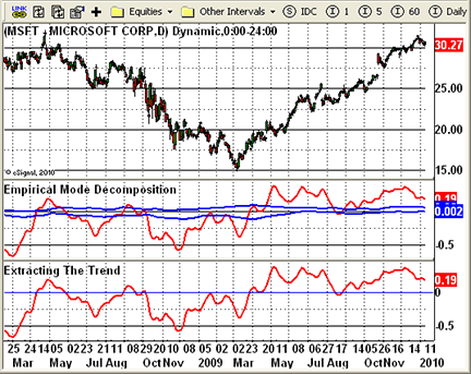
Figure 2: eSIGNAL, Empirical Mode Decomposition
![]() METASTOCK: EMPIRICAL MODE DECOMPOSITION
METASTOCK: EMPIRICAL MODE DECOMPOSITION
The article by John Ehlers and Ric Way in this issue, “Empirical Mode Decomposition,” presents three indicators. They can be added to MetaStock with the formulas listed here. To enter these indicators into MetaStock, follow these steps:
- In the Tools menu, select “Indicator Builder.”
- Click New to open the Indicator Editor for a new indicator.
- Type in the name “Bandpass.”
- Click in the larger window and paste or type in the following formula:
prd:=Input("number of periods",5,200,20);
dlta:=Input("Delta",0.01,5,0.1);
plot:=MP();

beta:=Cos(360/prd);
gam:=1/Cos((720*dlta)/prd);
alpha:=gam-Sqrt(gam*gam-1);
bp:=.5*(1-alpha)*(plot-Ref(plot,-2))+beta*(1+alpha)*PREV-alpha*Ref(PREV,-1);
bp
- Click OK to close the Indicator Editor.
- Click New to open the Indicator Editor for a new indicator.
- Type the name “Extracting the Trend.”
- Click in the larger window and paste or type in the formula.
prd:=Input("number of periods",5,200,20);
dlta:=Input("Delta",0.01,5,0.1);
plot:=MP();

beta:=Cos(360/prd);
gam:=1/Cos((720*dlta)/prd);
alpha:=gam-Sqrt(gam*gam-1);
bp:=.5*(1-alpha)*(plot-Ref(plot,-2))+beta*(1+alpha)*PREV-alpha*Ref(PREV,-1);
Mov(bp,2*prd,S)
- Click OK to close the Indicator Editor.
- Click New to open the Indicator Editor for a new indicator.
- Type in the name “Empirical Mode Decomposition.”
- Click in the larger window and paste or type in the following formula:
prd:=Input("number of periods",5,200,20);
dlta:=Input("Delta",0.01,5,0.1);
fra:=Input("fraction",0.01, 0.5, 0.1);
plot:=MP();

beta:=Cos(360/prd);
gam:=1/Cos((720*dlta)/prd);
alpha:=gam-Sqrt(gam*gam-1);
bp:=.5*(1-alpha)*(plot-Ref(plot,-2))+beta*(1+alpha)*PREV-alpha*Ref(PREV,-1);
pk:= If(Ref(bp,-1)>Max(bp,Ref(bp,-2)), Ref(bp,-1),PREV);
va:= If(Ref(bp,-1)<Min(bp,Ref(bp,-2)), Ref(bp,-1),PREV);
abp:=Mov(bp,2*prd,S);
apk:=Mov(pk,50,S);
ava:=Mov(va,50,S);
abp;
fra*apk;
fra*ava
- Click OK to close the Indicator Editor.
- Click OK to close Indicator Builder.
![]() WEALTH-LAB: EMPIRICAL MODE DECOMPOSITION
WEALTH-LAB: EMPIRICAL MODE DECOMPOSITION
For this month’s Traders’ Tip, we combined the ideas and indicators from “Empirical Mode Decomposition” by John Ehlers and Ric Way into a single script with a sample strategy in C# for Wealth-Lab 5.
While you can probably think of a dozen ways to use the cycle mode indicator and its thresholds, our sample strategy enters long trades when the cycle turns up within the threshold zone and exits on a closing profit of 4% or after five bars. The time-based exit was chosen purposely to be a quarter cycle in order to exit before the next downturn.
The strategy produced a slightly positive win rate and raw profit factor for the last six years of trading on the Dow Jones Industrial Average (Djia) and Nasdaq 100 index components (Figure 3)
.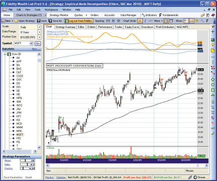
Figure 3: WEALTH-LAB, Empirical Mode Decomposition. Here are some representative trades from our sample Wealth-Lab strategy based on John Ehlers and Ric Way’s empirical mode decomposition method.
WealthScript code (C#):

using System;
using System.Collections.Generic;
using System.Text;
using System.Drawing;
using WealthLab;
using WealthLab.Indicators;

namespace WealthLab.Strategies
{
   public class EmpiricalModeDecomp : WealthScript
   {
      StrategyParameter _period;
      StrategyParameter _delta;
      StrategyParameter _fraction;

      public EmpiricalModeDecomp()
      {
         _period = CreateParameter("Period", 20, 5, 50, 1);
         _delta = CreateParameter("Delta", 0.5, 0.05, 1, 0.05);
         _fraction = CreateParameter("Fraction", 0.25, 0.1, 1, 0.05);
      }

      public DataSeries BandPassSeries(DataSeries ds, int period, double delta)
      {
         DataSeries res = new DataSeries(ds, "BandPassSeries(" + ds.Description + "," + period + "," + delta + ")");
         double beta = Math.Cos(2 * Math.PI / period);
         double gamma = 1/ Math.Cos(4 * Math.PI * delta / period);
         double alpha = gamma - Math.Sqrt(gamma * gamma - 1d);

         for (int bar = 2; bar < ds.Count; bar++)
         {
            res[bar] = 0.5 * (1 - alpha) * (ds[bar] - ds[bar - 2])
               + beta * (1 + alpha) * res[bar - 1] - alpha * res[bar - 2];
         }
         return res;
      }

      protected override void Execute()
      {
         int per = _period.ValueInt;
         double delta = _delta.Value;
         double fraction = _fraction.Value;

         DataSeries bp = BandPassSeries(AveragePrice.Series(Bars), per, delta);
         DataSeries ema = EMA.Series(Close, 100, EMACalculation.Modern);
         DataSeries mean = SMA.Series(bp, 2 * per);
         mean.Description = "SMA(" + bp.Description + "," + 2 * per + ")";
         DataSeries peak = new DataSeries(Bars, "peak()");
         DataSeries valley = new DataSeries(Bars, "valley()");
         double pk = 0d;
         double v = 0d;
         for(int bar = 2; bar < Bars.Count; bar++)
         {
            if( bp[bar-1] > bp[bar] && bp[bar-1] > bp[bar-2] )
               pk = bp[bar - 1];
            if( bp[bar-1] < bp[bar] && bp[bar-1] < bp[bar-2] )
               v = bp[bar-1];
            peak[bar] = pk;
            valley[bar] = v;
         }
         int avgPer = (int)(2.5 * per);
         DataSeries avgPeak = fraction * SMA.Series(peak, avgPer);
         DataSeries avgValley = fraction * SMA.Series(valley, avgPer);

         ChartPane cp = CreatePane( 40, true, false );
         DrawHorzLine(cp, 0d, Color.Black, LineStyle.Dashed, 1);
         PlotSeries(PricePane, ema, Color.Black, LineStyle.Solid, 1);
         PlotSeries(cp, avgPeak, Color.DodgerBlue, LineStyle.Solid, 1);
         PlotSeries(cp, avgValley, Color.DodgerBlue, LineStyle.Solid, 1);
         PlotSeries(cp, mean, Color.Orange, LineStyle.Solid, 2);

         /* Sample Trading Strategy */
         for (int bar = 2 * 100; bar < Bars.Count; bar++)
         {
            bool setup = mean[bar] > avgValley[bar]
               && mean[bar] < avgPeak[bar]
               && ema[bar] > ema[bar-1];

            if (IsLastPositionActive)
            {
               Position p = LastPosition;
               if (bar - p.EntryBar > 4)
                  SellAtMarket(bar + 1, p, "Time Based");
               else if (Close[bar] > p.EntryPrice * 1.04)
                  SellAtClose(bar, p, "Profit Target");
            }
            else if ( setup && TurnUp(bar, mean) )
            {
               SetBackgroundColor(bar, Color.LightCyan);
               BuyAtMarket(bar + 1);
            }
         }
      }
   }
}
![]() AMIBROKER: EMPIRICAL MODE DECOMPOSITION
AMIBROKER: EMPIRICAL MODE DECOMPOSITION
In “Empirical Mode Decomposition” in this issue, authors John Ehlers and Ric Way present an application of bandpass filtering to determine when the market is in cycle or trend modes.
Implementing bandpass filtering is easy in AmiBroker Formula Language. A ready-to-use formula based on the article is presented in Listing 1. To use it, enter the formula in the Afl editor, then press the “Insert indicator” button.
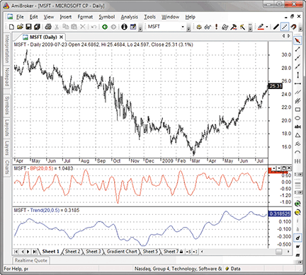
Figure 4: AMIBROKER, Empirical Mode Decomposition. Here is an example of cycle (middle pane) and trend (bottom pane) components for MSFT.
To display a chart similar to the one shown in Figure 4, press “Insert indicator” twice. This will create two chart panes. Then click on the chart with right mouse button and choose “Parameters” from the context menu to select the display mode: Choose either cycle or trend mode.
LISTING 1

SetBarsRequired( sbrAll );
PI = 3.1415926;

function Poly2ndOrder( input, N, c0, c1, b0, b1, b2, a1, a2 )
{
   output = input; // initialize for N first bars

  for( i = Max( N, 2 ); i < BarCount; i++ )
  {
     output[ i ] =   c0[ i ] * ( b0 * input[ i ] +
                                 b1 * input[ i - 1 ] +
                                 b2 * input[ i - 2 ] ) +
                     a1 * output[ i - 1 ] +
                     a2 * output[ i - 2 ] -
                     c1 * input[ i - N ];
  }

  return output;
}

function BandPass( input, Period, delta )
{
   N = 0;
   an = 2 * PI / Period;

   c0 = b0 = 1;
   c1 = b1 = b2 = a1 = a2 = gamma1 = 0;

   beta1 = cos( 2 * PI / Period );
   gamma1 = 1 / cos( 4 * PI * delta / Period );
   alpha = gamma1 - sqrt( gamma1 ^ 2 - 1 );
   a1 = beta1 * ( 1 + alpha );
   a2 = - alpha;

   c0 = ( 1 - alpha ) / 2;
   b2 = -1;

   return Poly2ndOrder( input, N, c0, c1, b0, b1, b2, a1, a2 );
}

Period = Param(“Period”, 20, 2, 100 );
Delta = Param(“Delta”, 0.5, 0.01, 1, 0.01 );

BP = BandPass( (H+L)/2, Period, Delta );
Trend = MA( BP, 2 * Period );

if( ParamToggle(“Mode”, “Cycle|Trend”, 0 ) == 0 )
 Plot( BP, “BP”+_PARAM_VALUES(), colorRed );
else
 Plot( Trend, “Trend”+_PARAM_VALUES(), colorBlue );
A sample chart is shown in Figure 4.
![]() WORDEN BROTHERS STOCKFINDER: EMPIRICAL MODE DECOMPOSITION
WORDEN BROTHERS STOCKFINDER: EMPIRICAL MODE DECOMPOSITION
The empirical mode decomposition setup described in “Empirical Mode Decomposition” by John Ehlers and Ric Way in this issue is easy to set up in StockFinder using RealCode.
You can add the indicator to your chart by clicking the “Add indicator/condition” button or by simply typing “/Empirical Mode” and choosing it from the list of available indicators.
Here is the code to display the empirical mode decomposition plot shown in Figure 5.
'# Cumulative
'# Period = UserInput.Integer = 20
'# Delta = UserInput.Single = 0.5
'# Fraction = UserInput.Single = 0.1
Static gamma As Single
Static alpha As Single
Static beta As Single
Static BP(2,2) As Single
Static Offset(2) As Integer
Static Trend As Single
Static Peak(1) As Single
Static Valley(1) As Single
Static AvgPeak As Single
Static AvgValley As Single
If isFirstBar Then
	beta = Math.Cos((360 / Period) * Math.PI / 180)
	gamma = 1 / Math.Cos((720 * delta / Period) * Math.PI / 180)
	alpha = gamma - ((gamma * gamma - 1) ^ .5)
	BP(2, 0) = 0
	BP(1, 0) = 0
	BP(0, 0) = 0
	BP(2, 1) = 0
	BP(1, 1) = 0
	BP(0, 1) = 0
	BP(2, 2) = 0
	BP(1, 2) = 0
	BP(0, 2) = 0
	Offset(0) = 2 * Period
	Offset(1) = Math.Max(Offset(0) + 1, 50)
	Offset(2) = Offset(0) + 2
	Trend = 0
	Peak(0) = 0
	Peak(1) = 0
	Valley(0) = 0
	Valley(1) = 0
	AvgPeak = 0
	AvgValley = 0
End If
If CurrentIndex >= 2 Then
	BP(2, 0) = BP(1, 0)
	BP(1, 0) = BP(0, 0)
	BP(0, 0) = .5 * (1 - alpha) * (Price.High + Price.Low _
		- Price.High(2) - Price.Low(2)) / 2 _
		+ beta * (1 + alpha) * BP(1, 0) - alpha * BP(2, 0)
	Trend += BP(0, 0) / Offset(0)
	If BP(1, 0) > BP(0, 0) AndAlso BP(1, 0) > BP(2, 0) Then Peak(0) = BP(1, 0)
	AvgPeak += Peak(0) / 50
	If BP(1, 0) < BP(0, 0) AndAlso BP(1, 0) < BP(2, 0) Then Valley(0) = BP(1, 0)
	AvgValley += Valley(0) / 50
	If CurrentIndex >= Offset(2) Then
		BP(2, 1) = BP(1, 1)
		BP(1, 1) = BP(0, 1)
		BP(0, 1) = .5 * (1 - alpha) * (Price.High(Offset(0)) + Price.Low(Offset(0)) _
			- Price.High(Offset(2)) - Price.Low(Offset(2))) / 2 _
			+ beta * (1 + alpha) * BP(1, 1) - alpha * BP(2, 1)
		Trend -= BP(0, 1) / Offset(0)
	End If
	If CurrentIndex >= 52 Then
		BP(2, 2) = BP(1, 2)
		BP(1, 2) = BP(0, 2)
		BP(0, 2) = .5 * (1 - alpha) * (Price.High(50) + Price.Low(50) _
			- Price.High(52) - Price.Low(52)) / 2 _
			+ beta * (1 + alpha) * BP(1, 2) - alpha * BP(2, 2)
		If BP(1, 2) > BP(0, 2) AndAlso BP(1, 2) > BP(2, 2) Then Peak(1) = BP(1, 2)
		AvgPeak -= Peak(0) / 50
		If BP(1, 2) < BP(0, 2) AndAlso BP(1, 2) < BP(2, 2) Then Valley(1) = BP(1, 2)
		AvgValley -= Valley(0) / 50
	End If
End If
If CurrentIndex >= Offset(1) Then
	OpenValue = Trend
	HighValue = Fraction * AvgPeak
	LowValue = Fraction * AvgValley
	Plot = Trend
Else
	OpenValue = Single.NaN
	HighValue = Single.NaN
	LowValue = Single.NaN
	Plot = Single.NaN
End If
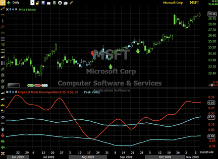
Figure 5: STOCKFINDER, Empirical Mode Decomposition. The empirical mode decomposition line is plotted along with peak and valley lines to identify when a stock is cycling (cyan price bars), entering an uptrend (green arrows), or entering a downtrend (red arrows).
RealCode is based on the Microsoft Visual Basic.Net framework and uses the Visual Basic (VB) language syntax. RealCode is compiled into a .Net assembly and run by the StockFinder application. RealCode is fully compiled and runs at the same machine-language level as the application itself, with the flexibility of run-time development and assembly that you get by writing your own custom code.
To use the indicators, rules and charts in this Traders’ Tip, you will need the StockFinder software. For more information or to start a free trial, please visit www.StockFinder.com.
![]() NEUROSHELL TRADER: EMPIRICAL MODE DECOMPOSITION
NEUROSHELL TRADER: EMPIRICAL MODE DECOMPOSITION
The bandpass filter and empirical mode decomposition indicators presented by John Ehlers and Ric Way in their article in this issue, “Empirical Mode Decomposition,” may be easily implemented in NeuroShell Trader by using a few of the program’s existing indicators and its ability to encode indicators in standard programming languages.
The bandpass filter indicator can be recreated in a standard programming language such as C, C++, Power Basic or Delphi. Convert the EasyLanguage code given in the article to a standard programming language of your choice and then insert the compiled result into your chart.
To recreate the empirical mode decomposition trend and threshold indicators from the bandpass filter (Figure 6), select “New Indicator…” from the Insert menu and use the Indicator Wizard to set up the following indicators:
BP:
BandPassFilter( Avg2( High, Low), 20, 0.5 )

Trend:
MovAvg ( BP, 40 )

Upper threshold:
Multiply2 ( 0.25 , MovAvg ( SelectiveLag ( Lag(BP,1) , And2( A>B( Lag(BP,1), BP ), A>B( Lag(BP,1), Lag(BP,2) ) ), 1 ), 50 ) )

Lower threshold:
Multiply2 ( 0.25 , MovAvg ( SelectiveLag ( Lag(BP,1) , And2( A<B( Lag(BP,1), BP ), A<B( Lag(BP,1), Lag(BP,2) ) ), 1 ), 50 ) )
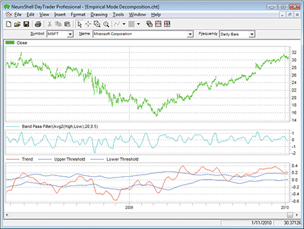
Figure 6: NEUROSHELL TRADER, Empirical Mode Decomposition. Here is a sample NeuroShell Trader chart showing the bandpass filter, trend, and empirical mode decomposition trend and threshold indicators.
You can create a dynamic trading system in NeuroShell Trader by combining the empirical mode decomposition trend and threshold indicators with NeuroShell Trader’s genetic algorithm optimizer to find optimal periods and fractions. Similar cycle-based strategies may also be recreated using the indicators found in John Ehlers’ Cybernetic and Mesa8 NeuroShell Trader Add-ons.
Users of NeuroShell Trader can go to the Stocks & Commodities section of the NeuroShell Trader free technical support website to download a copy of this or any past Traders’ Tips.
![]() AIQ: FLAT-BASE BREAKOUT SYSTEM
AIQ: FLAT-BASE BREAKOUT SYSTEM
The Aiq code is provided here for the flat-base breakout system, based on the January 2010 Stocks & Commodities article by Donald Pendergast, “The Search for Your Trading Style.” In the article, Pendergast uses a trend-following system as an example of a trading style. The rules for the system are as follows:
- Go long on the first 55-day “flat”-base breakout when volatility is falling during the base period
(using a seven-day average true range [Atr]) and the Chaikin money flow indicator is rising over the base period; - Exit long positions using a 3 Atr trailing stop.
After testing with only the above rules, I found that the trailing stop didn’t work very well to protect profits, so I added a profit-protect stop that becomes active once the profit has reached 5%. I decided to protect 90% of the profit. I also set up a buy-stop entry, which uses the prior 55-day high for the entry level. I also added minimum price and volume filters ($5.00 and 300,000 average daily shares). I also ensured that the 3 Atr trailing stop could never exceed the 20% value by adding a 20% trailing stop. All exits are based on the closing price and then are exited at the next day’s opening price.
This is a long-only system that I tested, using my entire database for the period December 31, 1998, to January 8, 2010. In Figure 7, I show the equity curve and metrics for a portfolio-trading simulation. During this period, there were 2,145 signals generated, of which about half were actually traded in the portfolio simulation once capitalization rules were added. The large drawdown from July 2007 to March 2009 indicates that the system might benefit from the addition of some simple market timing.
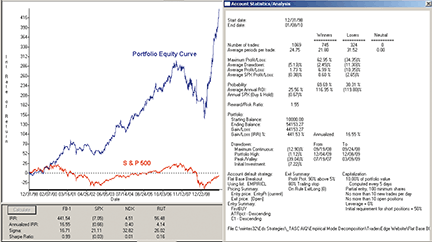
Figure 7: AIQ SYSTEMS, FLAT-BASE BREAKOUT SYSTEM. Here is a sample equity curve for the flat-base breakout system trading a portfolio of up to 10 simultaneous positions together with the related metrics for the period December 31, 1998, to January 8, 2010.
The code can be downloaded from the Aiq website at www.aiqsystems.com and also from www.tradersedgesystems.com/traderstips.htm.
! FLAT BASE BREAKOUT
! From the article named “The Search for Your Trading Style”
! Author: Donald Pendergast, TASC January 2010
! Coded by: Richard Denning 1/09/10
! www.TradersEdgeSystems.com

! Use built-in stops:
  ! Trailing set to 80%
  ! Profit protect set to protect 90% over 5%
  ! Also use trailing ATR exit rule below “ExitLong”
! Pricing:
  ! Entry pricing - “user defined = EntryPr and Current”
  ! Exit pricing - “Default (Next Period Open)”

! INPUTS
baseLen is 55.
bsATR	is 5.
stpATR	is 3.
atrLen	is 7.
cmfLen	is 100.
minPrice	is 5.
minVme	is 3000.

! ABBREVIATIONS:
C 	is [close].
C1 	is val([close],1).
O	is [open].
H	is [high].
L	is [low].
Name	is description().
OSD	is offSetToDate(month(),day(),year()).
PD 	is {Position days}.

! AVERAGE TRUE RANGE
TR 	is Max(H - L,max(abs(C1 - L),abs(C1- H))).
ATR	is simpleavg(TR,atrLen).
ATRpct	is simpleavg(TR / C,atrLen) * 100.

! BASE INDICATORS
HHbase	is highresult(H,baseLen,1).
HHdte	is scanany(H=^HHbase,baseLen+1).
HHos	is scanany(H=^HHbase,baseLen+1) then OSD.
LLbase	is lowresult(L,baseLen,1).
LLdte	is scanany(L=^LLbase,baseLen+1).
LLos	is scanany(L=^LLbase,baseLen+1) then OSD.
baseATR is (HHbase - LLbase) / ATR.
avgV	is simpleavg([volume],baseLen).

! CHAIKIN MONEY FLOW
AD	is [volume] * (C - O) / (H - L).
CMF	is sum(AD,cmfLen) / sum([volume],cmfLen).

! PRICE VOLUME AND DATA FILTER
PVD	if C > minPrice and avgV > minVme
	and hasdatafor(cmfLen+10) > baseLen.

! BREAKOUT RULE
BO	if H >  HHbase  and PVD.

! FLAT BASE RULE
FlatBase if (HHbase - LLbase) / ATR < bsATR and PVD.

! DECLINING VOLATILITY FILTER
VolaDwn	if slope2(ATR,baseLen) < 0 and PVD.

! INCREASING MONEYFLOW FILTER
MFup	if slope2(CMF,baseLen) > 0 and PVD.

! ENTRY RULE
Buy 	if  (HHbase - LLbase) / ATR < bsATR
	and H >  HHbase
	and slope2(ATR,baseLen) < 0
	and slope2(CMF,baseLen) > 0
	and PVD.

! ENTRY RULE RESTRICTED TO FIRST BREAK OUT IN LAST 10 BARS
FirstBUY if Buy and countof(BO,10) = 1.

! ENTRY PRICE
EntryPr	is max(O,HHbase).

! TRAILING EXIT
stop 	is L - ATR * stpATR.
stopVal	is highresult(stop,PD,1).
ExitLong if C < stopVal.
![]() TRADERSSTUDIO: EMPIRICAL MODE DECOMPOSITION
TRADERSSTUDIO: EMPIRICAL MODE DECOMPOSITION
The TradersStudio code is provided here to help implement the ideas and indicators presented in “Empirical Mode Decomposition” by John Ehlers and Ric Way.
I have supplied the indicator code as well as the code for a simple system (described below) that I devised to test the indicator. In Figure 8, I show the three indicators as they appear on an optimized chart of Spy. The indicator looks different than the examples shown in Ehlers and Way’s article because I changed the parameters based on an optimization.
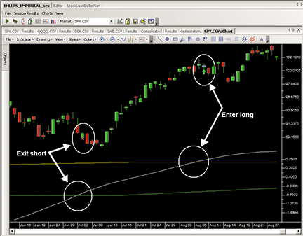
Figure 8: TRADERSSTUDIO, Empirical INDICATOR. Here is an implementation of the empirical indicator with an exit and entry signal.
I created a simple system to test the indicator and then used it to find the appropriate range of parameters. In Figure 8, I am using parameters of period = 85, delta = 0.4, and fraction = 0.1, which represent one of the better parameter sets for the following system, which trades only when the indicator is in the trending mode and steps aside when in the cycle mode:
- Go long when the mean of the empirical indicator crosses over the upper band (AvgPeak)
- Exit long when the mean crosses down under the upper band
- Go short when the mean crosses under the lower band (AvgValley)
- Exit short when the mean crosses over the lower band.
In Figure 9, I show a three-dimensional parameter-optimization map for the above system. The most sensitive parameter is fraction, which is the one that sets the upper and lower bands. The right-most parameter map in Figure 9 shows that this parameter is very sensitive and likes a very small value between 0.05 and 0.1, with larger values degrading rapidly. The other two parameters are more robust. In Figure 10, I show the resulting equity curve based on trading equal dollar amounts of Spy, Dia, Qqqq, and Iwb for the period June 2002 to December 2009.
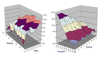
Figure 9: TRADERSSTUDIO, 3D PARAMETER MAP. Here is a three-dimensional parameter map for a trend-following system that uses the empirical indicator to signal trades.
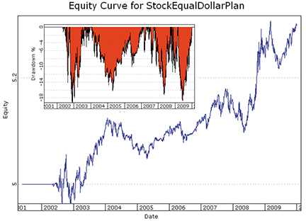
Figure 10: TRADERSSTUDIO, EQUITY CURVES. Here are log equity (blue) and underwater equity (red) curves trading a portfolio of four ETFs (SPY, DIA, QQQQ, IWB) for the period June 2002 to December 2009.
The code can be downloaded from the TradersStudio website at www.TradersStudio.com → Traders Resources → FreeCode and also from www.TradersEdgeSystems.com/traderstips.htm.
![]() TRADINGSOLUTIONS: EMPIRICAL MODE DECOMPOSITION
TRADINGSOLUTIONS: EMPIRICAL MODE DECOMPOSITION
In “Empirical Mode Decomposition” in this issue, authors John Ehlers and Ric Way present a bandpass filter for use as a cycle- and trend-detection indicator.
These functions are described here and are also available as a function file that can be downloaded from the TradingSolutions website (www.tradingsolutions.com) in the “Free Systems” section.
Function Name: Ehlers Bandpass Filter Beta
Short Name: EBPF_Beta
Inputs: Period
Cos (Div (360, Period))

Function Name: Ehlers Bandpass Filter Gamma
Short Name: EBPF_Gamma
Inputs: Period, Delta
Div (1, Cos (Div (Mult (720, Delta), Period)))

Function Name: Ehlers Bandpass Filter Alpha
Short Name: EBPF_Alpha
Inputs: Period, Delta
Sub (EBPF_Gamma (Period, Delta), Sqrt (Sub (Pow (EBPF_Gamma (Period, Delta), 2), 1)))

Function Name: Ehlers Bandpass Filter
Short Name: EBPF
Inputs: Price, Period, Delta
Sub (Add (Mult (0.5, Mult (Sub (1, EBPF_Alpha (Period, Delta)), Sub (Price, Lag (Price, 2)))), Mult (Mult (EBPF_Beta (Period), Add (1, EBPF_Alpha (Period, Delta))), Prev (1))), Mult (EBPF_Alpha (Period, Delta), Prev (2)))

Function Name: Ehlers Bandpass Filter Trend
Short Name: EBPF_Trend
Inputs: Price, Period, Delta
Div (Add (MA (EBPF (Price, Period, Delta), Period), Lag (MA (EBPF (Price, Period, Delta), Period), Period)), 2)
Function Name: Ehlers Bandpass Filter Peak
Short Name: EBPF_Peak
Inputs: Price, Period, Delta
If (And (GT (Lag (EBPF (Price, Period, Delta), 1), EBPF (Price, Period, Delta)), GT (Lag (EBPF (Price, Period, Delta), 1), Lag (EBPF (Price, Period, Delta), 2))), Lag (EBPF (Price, Period, Delta), 1), Prev (1))

Function Name: Ehlers Bandpass Filter Valley
Short Name: EBPF_Valley
Inputs: Price, Period, Delta
If (And (LT (Lag (EBPF (Price, Period, Delta), 1), EBPF (Price, Period, Delta)), LT (Lag (EBPF (Price, Period, Delta), 1), Lag (EBPF (Price, Period, Delta), 2))), Lag (EBPF (Price, Period, Delta), 1), Prev (1))

Function Name: Ehlers Bandpass Filter Upper Threshold
Short Name: EBPF_Upper
Inputs: Price, Period, Delta, Fraction, Threshold Period
Mult (Fraction, MA (EBPF_Peak (Price, Period, Delta), Threshold Period))

Function Name: Ehlers Bandpass Filter Lower Threshold
Short Name: EBPF_Lower
Inputs: Price, Period, Delta, Fraction, Threshold Period
Mult (Fraction, MA (EBPF_Valley (Price, Period, Delta), Threshold Period))
![]() TRADECISION: EMPIRICAL MODE DECOMPOSITION
TRADECISION: EMPIRICAL MODE DECOMPOSITION
The article by John Ehlers and Ric Way in this issue, “Empirical Mode Decomposition,” demonstrates a unique approach to market research based on the cycling and trend modes. It also addresses trading accordingly after the market mode has been identified.
You can recreate several of the indicators using Tradecision’s Indicator Builder with the following code:
BANDPASS FILTER indicator:
input
Price:”Enter the Price:”, MedianPrice;
Period:”Enter the Period:”, 20;
Delta:”Enter the Delta:”, 0.1;
end_input

var
gamma:=0;
alpha:=0;
beta:=0;
BP1:=0;
BP2:=0;
BP:=0;
end_var

if HistorySize < period + 2 then return 0;

beta:=Cos(360 / Period);
gamma:=1 / Cos(720 * delta / Period);
alpha:=gamma - SquareRoot(gamma * gamma - 1);
BP1:=0.5 * (1 - alpha) * (Price - Price\2\);
BP2:=BP1 + beta * (1 + alpha) * BP1\1\ ;
BP:=BP2 - alpha * BP1\2\;

return BP;

EXTRACTING THE TREND indicator:
input
Price:”Enter the Price:”, MedianPrice;
Period:”Enter the Period:”, 20;
Delta:”Enter the Delta:”, 0.1;
end_input

var
gamma:=0;
alpha:=0;
beta:=0;
BP1:=0;
BP2:=0;
BP:=0;
Trend:=0;
end_var

if HistorySize < period + 2 then return 0;

(360 / Period);
gamma:=1 / Cos(720 * delta / Period);
alpha:=gamma - SquareRoot(gamma * gamma - 1);
BP1:=0.5 * (1 - alpha) * (Price - Price\2\);
BP2:=BP1 + beta * (1 + alpha) * BP1\1\ ;
BP:=BP2 - alpha * BP1\2\;
Trend:=SMA(BP, 2 * Period);

return Trend;

EMPIRICAL MODE DECOMPOSITION PEAK indicator:
input
Price:”Enter the Price:”, MedianPrice;
Period:”Enter the Period:”, 20;
Delta:”Enter the Delta:”, 0.5;
Fraction:”Enter the Fraction:”, 0.1;
end_input

var
alpha:=0;
beta:=0;
gamma:=0;
BP1:=0;
BP2:=0;
BP:=0;
Peak:=0;
AvgPeak:=0;
end_var

beta:=Cos(360 / Period);
gamma:=1 / Cos(720 * delta / Period);
alpha:=gamma - SquareRoot(gamma * gamma - 1);
BP1:=0.5 * (1 - alpha) * (Price - Price\2\);
BP2:=BP1 + beta * (1 + alpha) * BP1\1\ ;
BP:=BP2 - alpha * BP1\2\;

if BP\1\ > BP and BP\1\ > BP\2\ then Peak:=BP\1\;
AvgPeak:=SMA(Peak, 50);

return Fraction * AvgPeak;

EMPIRICAL MODE DECOMPOSITION VALLEY indicator:
input
Price:”Enter the Price:”, MedianPrice;
Period:”Enter the Period:”, 20;
Delta:”Enter the Delta:”, 0.5;
Fraction:”Enter the Fraction:”, 0.1;
end_input

var
alpha:=0;
beta:=0;
gamma:=0;
BP1:=0;
BP2:=0;
BP:=0;
Valley:=0;
AvgValley:=0;
end_var

if HistorySize < period + 2 then return 0;

beta:=Cos(360 / Period);
gamma:=1 / Cos(720 * delta / Period);
alpha:=gamma - SquareRoot(gamma * gamma - 1);
BP1:=0.5 * (1 - alpha) * (Price - Price\2\);
BP2:=BP1 + beta * (1 + alpha) * BP1\1\ ;
BP:=BP2 - alpha * BP1\2\;

if BP\1\ < BP and BP\1\ < BP\2\ then Valley:=BP\1\;
AvgValley:=SMA(Valley, 50);

return Fraction * AvgValley;
To import this strategy into Tradecision, visit the area “Traders’ Tips from Tasc Magazine” at www.tradecision.com/support/tasc_tips/tasc_traders_tips.htm or copy the code from the Stocks & Commodities website at www.traders.com.
A sample chart is shown in Figure 11.
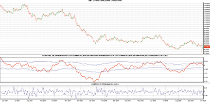
FIGURE 11: TRADECISION, BANDPASS FILTER AND TREND WITH MODE THRESHOLDS (Fraction = 0.2). If the trend is above the upper threshold, then the market is considered to be in an uptrend. If the trend is below the lower threshold, then the market is in a downtrend. When the trend falls between the two threshold levels, the market is in a cycle mode.
![]() NINJATRADER: EMPIRICAL MODE DECOMPOSITION
NINJATRADER: EMPIRICAL MODE DECOMPOSITION
The empirical mode decomposition indicator, discussed in “Empirical Mode Decomposition” by John Ehlers and Ric Way in this issue, has been implemented as an indicator available for download at www.ninjatrader.com/SC/March2010SC.zip.
Once it has been downloaded, from within the NinjaTrader Control Center window, select the menu File → Utilities → Import NinjaScript and select the downloaded file. This indicator is for NinjaTrader version 6.5 or greater.
You can review the indicator’s source code by selecting the menu Tools → Edit NinjaScript → Indicator from within the NinjaTrader Control Center window and selecting EmpiricalModeDecomposition.
NinjaScript indicators are compiled Dlls that run native, not interpreted, which provides you with the highest performance possible.
A sample chart implementing the strategy is shown in Figure 12.
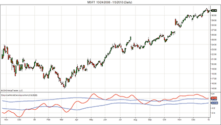
Figure 12: NINJATRADER, Empirical Mode Decomposition. This screenshot shows the empirical mode decomposition indicator applied to a daily chart of Microsoft (MSFT).
![]() NEOTICKER: EMPIRICAL MODE DECOMPOSITION
NEOTICKER: EMPIRICAL MODE DECOMPOSITION
The indicators described by John Ehlers and Ric Way in their article in this issue, “Empirical Mode Decomposition,” can be implemented in NeoTicker using NeoTicker’s formula language.
The three indicators presented in the article are the bandpass filter (Listing 1); extracting the trend (Listing 2); and empirical mode decomposition (Listing 3).
The bandpass filter and extracting the trend indicators have two parameters: period and delta. They plot an oscillator along with a zero line in a new pane. The empirical mode decomposition has three parameters: period, delta, and fraction. It returns three plots in a new pane. An example of the three indicators applied to a daily Msft chart is shown in Figure 13.
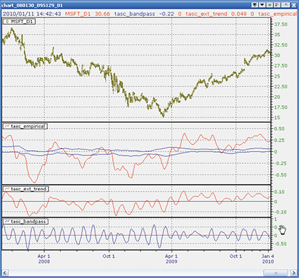
Figure 13: NEOTICKER, Empirical Mode Decomposition STRATEGY
One additional function, deg2rad, is added to simulate the calculation results from EasyLanguage, which was used in the article. The deg2rad function is needed because the cosine calculation in EasyLanguage returns degrees instead of radians like most conventional math programs do.
Code for all three indicators will be available for download at the NeoTicker blog site (https://blog.neoticker.com).
LISTING 1
myprice := (h+l)/2;
$period := param1;
$delta := param2;
$beta  := cos (deg2rad (360 / $period));
$gamma := 1 / cos (deg2rad (720 * $delta / $period));
$alpha := $gamma - sqrt ($gamma * $gamma - 1);
BP := 0.5*(1-$alpha)*(myprice-myprice(2))+$beta*(1+$alpha)*BP(1)-$alpha*BP(2);
plot1 := BP;
plot2 := 0;

LISTING 2
myprice := (h+l)/2;
$period := param1;
$delta := param2;
$beta  := cos (deg2rad (360 / $period));
$gamma := 1 / cos (deg2rad (720 * $delta / $period));
$alpha := $gamma - sqrt ($gamma * $gamma - 1);
BP := 0.5*(1-$alpha)*(myprice-myprice(2))+$beta*(1+$alpha)*BP(1)-$alpha*BP(2);
plot1 := average(BP, 2*$period);
plot2 := 0;

LISTING 3
myprice := (h+l)/2;
$period := param1;
$delta := param2;
$fraction := param3;
$beta  := cos (deg2rad (360 / $period));
$gamma := 1 / cos (deg2rad (720 * $delta / $period));
$alpha := $gamma - sqrt ($gamma * $gamma - 1);
BP := 0.5*(1-$alpha)*(data1-data1(2))+$beta*(1+$alpha)*BP(1)-$alpha*BP(2);
Peak := if((BP(1) > BP) and (BP(1) > BP(2)), BP(1), Peak);
Valley := if((BP(1) < BP) and (BP(1) < BP(2)), BP(1), Valley);
plot1 := average(BP, 2*$period);
plot2 := $fraction*average(Peak, 50);
plot3 := $fraction*average(Valley, 50);
![]() WAVE59: EMPIRICAL MODE DECOMPOSITION
WAVE59: EMPIRICAL MODE DECOMPOSITION
In “Empirical Mode Decomposition” in this issue, authors John Ehlers and Ric Way present an objective method for determining whether the market is in trend mode or cycle mode.
Figure 14 is a daily chart of the Dow Jones Industrial Average showing their cycle indicator at work. We’ve enhanced their initial code to color the bars based on what mode the market is in: red means a downward-trending market, blue is an upward-trending market, and black is cycle mode. Notice how the recent upmove was built on a combination of blue upward-trending thrusts plus black cyclical retracements.
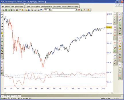
FIGURE 14: WAVE59, Empirical Mode Decomposition. The cycle indicator is shown here on a daily chart of the Dow Jones Industrial Average. Red indicates a downtrending market, blue an uptrending market, and black is cycle mode.
The following script implements this indicator in Wave59. As always, users of Wave59 can download these scripts directly using the QScript Library found at https://www.wave59.com/library.
Indicator:  Ehlers_EmpiricalModeDecomposition
input:price( (high+low)/2 ), period(20), delta(0.1), fraction(0.1), color(red), threshcolor(blue);

# initialization block
if (barnum == barsback) {
    bp, peak, valley=0;
}

#compute trend
beta = cos(360/period);
gamma = 1/cos(720*delta/period);
alpha = gamma - sqrt(gamma*gamma - 1);
bp=0.5*(1-alpha)*(price-price[2])  +  beta*(1+alpha)*bp[1]  -  alpha*bp[2];
mean=average(bp, 2*period);

# compute thresholds
peak = peak[1];
valley = valley[1];
if (bp[1]>bp and bp[1]>bp[2]) peak = bp[1];
if (bp[1]<bp and bp[1]<bp[2]) valley = bp[1];
avgpeak = average(peak, 50);
avgvalley = average(valley, 50);

# plot it
plot1 = mean;
color1 = color;
plot2 = fraction*avgpeak;
plot3 = fraction*avgvalley;
color2, color3 = threshcolor;
style2, style3 = ps_dot;

# colorbars
if (mean>fraction*avgpeak) colorbar(barnum, blue, 1);
if (mean<fraction*avgvalley) colorbar(barnum, red, 1);
![]() VT TRADER: EMPIRICAL MODE DECOMPOSITION
VT TRADER: EMPIRICAL MODE DECOMPOSITION
This Traders’ Tip is based on the article by John Ehlers and Ric Way in this issue, “Empirical Mode Decomposition.” We will be offering the empirical mode decomposition (Emd) indicator for download in our online forums. The VT Trader code and instructions for recreating the indicator in VT Trader are as follows:
- VT Trader’s Ribbon → Technical Analysis menu → Indicators group → Indicators Builder → [New] button
- In the General tab, type the following text into each corresponding text box:
Name: TASC - 03/2010 - Empirical Mode Decomposition
Function Name Alias: tasc_EMD
Label Mask: TASC - 03/2010 - Empirical Mode Decomposition (%Price%,%Period%,%d%,%Fraction%)
Mean = %Mean%, Upper Band = %Upper_Threshold%, Lower Band = %Lower_Threshold%
Placement: New Frame
Data Inspection Alias: EMD
- In the Input Variable(s) tab, create the following variables:
[New] button...
Name: Price
Display Name: Price
Type: price
Default: Median Price

[New] button...
Name: Period
Display Name: Periods
Type: integer
Default: 20

[New] button...
Name: d
Display Name: Delta
Type: float
Default: 0.5

[New] button...
Name: Fraction
Display Name: Fraction
Type: float
Default: 0.1
- In the Output Variable(s) tab, create the following variables:
[New] button...
Var Name: Mean
Name: (Mean)
Line Color: dark red
Line Width: slightly thicker
Line Type: solid

[New] button...
Var Name: Upper_Threshold
Name: (Upper Threshold)
Line Color: blue
Line Width: slightly thicker
Line Type: solid

[New] button...
Var Name: Lower_Threshold
Name: (Lower Threshold)
Line Color: blue
Line Width: slightly thicker
Line Type: solid
- In the Formula tab, copy and paste the following formula:
{Provided By: Capital Market Services, LLC & Visual Trading Systems, LLC}
{Copyright: 2010}
{Description: TASC, March 2010 - “Cycle Vs. Trend Mode Detection - Empirical Mode Decomposition” by John F. Ehlers and Ric Way}
{File: tasc_EMD.vtscr - Version 1.0}
b:= cos(360/Period);
g:= 1/cos(720*d/Period);
a:= g-sqrt(g*g-1);
BP:= if(IsDefined(BP)=0,0,BP);
BP:= 0.5*(1-a)*(Price-ref(Price,-2))+b*(1+a)*ref(BP,-1)-a*ref(BP,-2);
Mean:= mov(BP,2*Period,S);
_Peak:= if(ref(BP,-1)>BP and ref(BP,-1)>ref(BP,-2),ref(BP,-1),PREV(0));
_Valley:= if(ref(BP,-1)<BP and ref(BP,-1)<ref(BP,-2),ref(BP,-1),PREV(0));
AvgPeak:= mov(_Peak,50,S);
AvgValley:= mov(_Valley,50,S);
Upper_Threshold:= Fraction*AvgPeak;
Lower_Threshold:= Fraction*AvgValley;
- Click the “Save” icon in the toolbar to finish building the EMD indicator.
To attach the indicator to a chart, click the right mouse button within the chart window and then select “Add Indicator” → “TASC - 03/2010 - Empirical Mode Decomposition” from the indicator list.
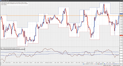
Figure 15: VT TRADER, Empirical Mode Decomposition. Here is an example of the EMD indicator on a EUR/USD one-hour candlestick chart.
To learn more about VT Trader, visit www.cmsfx.com.
Risk disclaimer: Past performance is not indicative of future results. Forex trading involves a substantial risk of loss and may not be suitable for all investors.
![]() EASYLANGUAGE: EMPIRICAL MODE DECOMPOSITION — ARTICLE CODE
EASYLANGUAGE: EMPIRICAL MODE DECOMPOSITION — ARTICLE CODE
Below is the code from John Ehlers and Ric Way’s article in this issue, “Empirical Mode Decomposition.”
BANDPASS FILTER CODE IN EASYLANGUAGE
Inputs:
	Price((H+L)/2),
	Period(20),
	delta(.1);

Vars:
	gamma(0),
	alpha(0),
	beta(0),
	BP(0);

beta = Cosine(360 / Period);
gamma = 1 / Cosine(720*delta / Period);
alpha = gamma - SquareRoot(gamma*gamma - 1);
BP = .5*(1 - alpha)*(Price - Price[2]) + beta*(1 + alpha)*BP[1]- alpha*BP[2];

Plot1(BP);
Plot2(0);

EXTRACTING THE TREND IN EASYLANGUAGE
Inputs:
	Price((H+L)/2),
	Period(20),
	Delta(.1);

Vars:
	gamma(0),
	alpha(0),
	beta(0),
	BP(0),
	Trend(0);

beta = Cosine(360 / Period);
gamma = 1 / Cosine(720*delta / Period);
alpha = gamma - SquareRoot(gamma*gamma - 1);
BP = .5*(1 - alpha)*(Price - Price[2]) + beta*(1 + alpha)*BP[1] - alpha*BP[2];
Trend = Average(BP, 2*Period);

Plot1(Trend);
Plot2(0);


EMPIRICAL MODE DECOMPOSITION IN EASYLANGUAGE
Inputs:
	Price((H+L)/2),
	Period(20),
	delta(.5),
	Fraction(.1);

Vars:
	alpha(0),
	beta(0),
	gamma(0),
	BP(0),
	I(0),
	Mean(0),
	Peak(0),
	Valley(0),
	AvgPeak(0),
	AvgValley(0);

beta = Cosine(360 / Period);
gamma = 1 / Cosine(720*delta / Period);
alpha = gamma - SquareRoot(gamma*gamma - 1);
BP = .5*(1 - alpha)*(Price - Price[2]) + beta*(1 + alpha)*BP[1] - alpha*BP[2];
Mean = Average(BP, 2*Period);
Peak = Peak[1];
Valley = Valley[1];
If BP[1] > BP and BP[1] > BP[2] Then Peak = BP[1];
If BP[1] < BP and BP[1] < BP[2] Then Valley = BP[1];

AvgPeak = Average(Peak, 50);
AvgValley = Average(Valley, 50);

Plot1(Mean);
Plot2(Fraction*AvgPeak);
Plot6(Fraction*AvgValley);